Principal components regression

Principal components analysis (PCA) is a common and popular technique for deriving a low-dimensional set of features from a large set of variables. For more information on PCA, please refer to my earlier post on the technique. In this post, I’ll explore using PCA as a dimension reduction technique for regression, known as principal components regression.

The structure of this post was influenced by the sixth chapter of An Introduction to Statistical Learning: with Applications in R by Gareth James, Daniela Witten, Trevor Hastie, and Robert Tibshirani.

Principal components regression

Principal components regression (PCR) involves first performing principal components analysis on our data set to obtain the first $M$ principal components $Z_1, \ldots, Z_M$. These components are then used as the predictors in a linear regression model fit using least squares.

The underlying idea behind PCR is that often a small number of principal components can sufficiently explain most of the variability in the data, as well as the predictor’s relationship with the response. Thus, we assume that the directions in which $X_1, \ldots, X_p$ show the most variation are the directions that are associated with $Y$. This assumption is often not guaranteed, but does turn out to be a reasonable enough approximation and provide good results. If the assumption does hold, then fitting a least squares model to $Z_1, \ldots, Z_M$ will lead to better results that fitting a least squares model to $X_1, \ldots, X_p$, and we will also be able to mitigate overfitting. As with PCA, it is recommended to standardize each predictor before performing PCR.

For clarity, we use the actual principal component scores when performing principal components regression. Just as when performing ordinary linear regression with one predictor, we fit $Y$ onto $X_1$ where $X_1$ is a vector containing the values $x_1, x_2, \ldots, x_n$, when performing PCR with one principal components we fit $Y$ onto $Z_1$ where $Z_1$ is a vector containing the principal component scores $z_1, z_2, \ldots, z_n$.

import pandas as pd
import seaborn as sns
from sklearn.datasets import load_diabetes
from sklearn.decomposition import PCA
from sklearn.linear_model import LinearRegression
from sklearn.model_selection import cross_val_score
from sklearn.preprocessing import StandardScaler

# Loading data as NumPy arrays
X, y = load_diabetes(return_X_y=True)

# Initializing estimator
standard_scaler = StandardScaler()

# Scaling predictors
X = standard_scaler.fit_transform(X)

# Initializing estimator
pca = PCA()

# Performing PCA
pc_scores = pca.fit_transform(X)

# Initializing estimator
lin_reg = LinearRegression()

# Creating lists to hold results
components_used = []
mean_squared_errors = []

# Performing 10-fold cross validation on sequential amount of principal components
for i in range(1, 11):

    # 10-fold cross-validation
    cv_scores = cross_val_score(estimator=lin_reg,
                                X=pc_scores[:, 0:i],
                                y=y,
                                cv=10,
                                scoring="neg_mean_squared_error")

    # Calculating average of negative mean squared error, and turning positive
    # Note: scikit-learn offers negative MSE because cross_val_score attempts to maximize a scoring metric
    # Since we want a low MSE, we want a high negative MSE
    cv_mean_squared_error = cv_scores.mean() * -1

    # Appending results
    components_used.append(i)
    mean_squared_errors.append(cv_mean_squared_error)

# Organizing cross-validation results into DataFrame
mse_by_n_components = \
    pd.DataFrame(data=dict(components_used=components_used,
                           mean_squared_errors=mean_squared_errors))

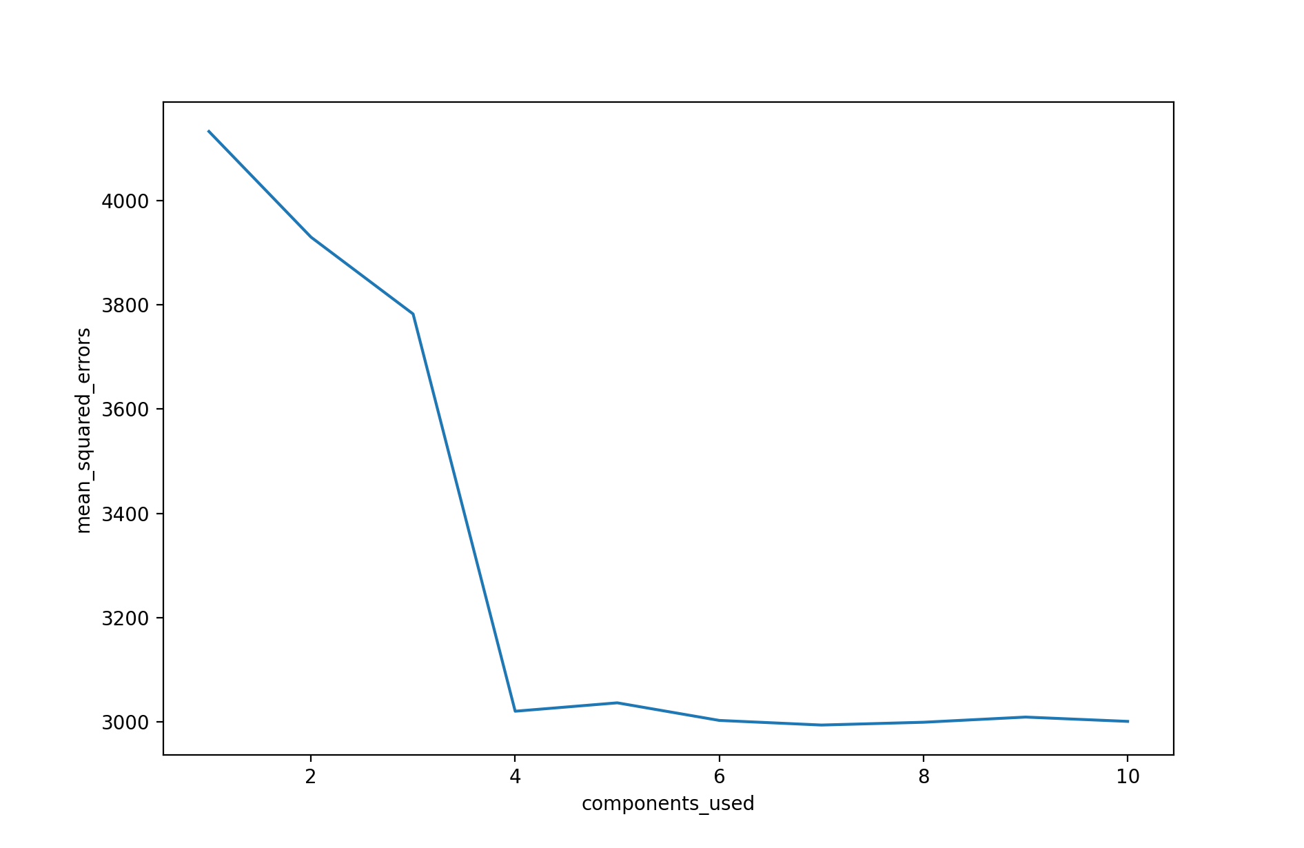
In the above plot, we see the results of PCR applied to the common Diabetes dataset. The resulting test mean squared error (MSE) estimate from each fit is plotted against the number of principal components used in that fit. From the plot, we see a strong decrease in the test MSE estimate when four principal components are used, and then a leveling off as further principal components are used. The absolute minimum test MSE estimate occurs when seven principal components are used. As more principal components are used in the regression model, the bias decreases, but the variance increases, causing the sharp decrease and eventual increase in the plot. Of course, when the number of components $M$ used is equivalent to the number of predictor variables $p$, then PCR is simply the least squares fit using all of the original predictors.

The above plot indicates that PCR performed with an appropriate choice of $M$ can lead to a significant improvement over least squares. This is especially true when much of the variability and association with the response are contained in a small number of the predictors. In contrast, PCR will tend to not perform as well when many principal components are needed to adequately model the response. In some situations, PCR may outperform shrinkage methods, such as ridge regression and the lasso, and in other situations it may not. For any given use case, model performance evaluation is needed to determine the best performing model.

Note, PCR is not a feature selection method. This is because each of the $M$ principal components used in the regression model is a linear combination of all of the original predictors $p$. Thus, PCR is more closely related to ridge regression than the lasso.

Choosing the number of principal components

In contrast to principal components analysis, which is inherently an unsupervised approach, PCR is a supervised approached. In PCR, the number of principal components $M$ is typically chosen via cross-validation. A method such as $k$-fold cross-validation or leave-one-out cross-validation should be used.