This is the second post in a short series discussing the common regularization methods of ridge regression and the lasso. In an earlier post, I introduced much of the theory surrounding these methods. For a more detailed overview of regularization, please see that earlier post.
In this post, I’ll explore examples of ridge regression and the lasso using both scikit-learn and statsmodels. scikit-learn’s implementation of these two particular methods is more robust, so I’ll spend most of the below post discussing and using that package.
Boston housing dataset
For the below examples, I’ll use the common Boston housing dataset, available via scikit-learn.
from sklearn.datasets import load_boston

# Loading boston housing data
X, y = load_boston(return_X_y=True)
Scaling features
When performing regularization, it’s important to scale our predictors. For regularization, we do not have to scale our response variable, but it doesn’t hurt to do so either. Below I’ll just scale the array of predictors X.
from sklearn.preprocessing import StandardScaler

# Scaling input features
standard_scaler = StandardScaler()
X = standard_scaler.fit_transform(X)
Ridge regression
To begin, I’ll simply perform ridge regression using scikit-learn’s Ridge estimator. We can control the penalty term of our ridge regression using the alpha parameter. This parameter is often denoted as $\lambda$ in the statistical literature.
from sklearn.linear_model import Ridge

# Initializing Ridge estimator, defining lambda (alpha) to be 0.1
ridge_reg = Ridge(alpha=0.1)

# Fitting estimator
ridge_reg.fit(X, y)

# Viewing results
ridge_reg.score(X, y)  # training R^2 square
ridge_reg.coef_        # coefficients
ridge_reg.intercept_   # intercept
ridge_reg.predict(X)   # getting predictions
$k$-fold cross-validation
To better evaluate how our above ridge regression model is perform when alpha=0.1, we can perform $k$-fold cross-validation using cross_val_score.
# Using cross_val_score (evaluating model on mean and std of R^2 values)
from sklearn.model_selection import cross_val_score

# Initializing cross_val_score estimator, 5-fold cross-validation
cv_scores = cross_val_score(estimator=ridge_reg, X=X, y=y, cv=5)

# Mean and standard deviation of training scores across folds
cv_scores.mean()
cv_scores.std()
Determining optimal alpha via GridSearchCV
To determine an ideal value of alpha, we can use scikit-learn’s GridSearchCV. This estimator takes a grid of candidate alpha values and performs cross-validation to determine which value is performing the best. Of course, other parameters can be evaluated using GridSearchCV as well.
Below, we find the best ridge regression performance occurs when alpha=100.
import numpy as np
from sklearn.model_selection import GridSearchCV

# Defining grid of candidate alpha values (powers of 10, from 0.00001 to 1000000)
param_grid = {"alpha": 10.0 ** np.arange(-5, 6)}

# Initializing Ridge and GridSearchCV estimators
ridge_reg = Ridge()
grid_search = GridSearchCV(estimator=ridge_reg, param_grid=param_grid)

# Fitting grid search object
grid_search.fit(X, y)

# Results
grid_search.best_params_     # best alpha=100
grid_search.best_estimator_  # best estimator object
grid_search.best_score_      # highest mean 5-fold cross-validated test score (corresponds where alpha=100)

grid_search.predict(X)       # predictions using best model, refit on all folds
grid_search.score(X, y)      # training score of best model, refit on all folds
We can view detailed results of our grid search by converting the cv_results_ attribute into a pandas DataFrame.
>>> import pandas as pd

# Detailed results as pandas DataFrame
>>> grid_search_results = pd.DataFrame(grid_search.cv_results_)
grid_search_results

   mean_fit_time  std_fit_time  mean_score_time  std_score_time   param_alpha               params  split0_test_score  split1_test_score  split2_test_score  split3_test_score  split4_test_score  mean_test_score  std_test_score  rank_test_score
0        0.006385      0.006901         0.004554        0.007661       0.00001     {'alpha': 1e-05}           0.639200           0.713867           0.587023           0.079231          -0.252941         0.353276        0.376568                8
1        0.017601      0.028352         0.003629        0.004682       0.00010    {'alpha': 0.0001}           0.639200           0.713867           0.587024           0.079231          -0.252939         0.353277        0.376567                7
2        0.001465      0.000604         0.000752        0.000305       0.00100     {'alpha': 0.001}           0.639204           0.713870           0.587025           0.079234          -0.252914         0.353284        0.376560                6
3        0.001402      0.000858         0.000619        0.000155       0.01000      {'alpha': 0.01}           0.639242           0.713898           0.587035           0.079260          -0.252668         0.353353        0.376489                5
4        0.001348      0.000379         0.000798        0.000377       0.10000       {'alpha': 0.1}           0.639623           0.714174           0.587142           0.079524          -0.250222         0.354048        0.375788                4
5        0.000600      0.000028         0.000365        0.000050       1.00000       {'alpha': 1.0}           0.643330           0.716837           0.588143           0.082143          -0.227025         0.360686        0.369177                3
6        0.000586      0.000014         0.000340        0.000002      10.00000      {'alpha': 10.0}           0.672352           0.735087           0.593675           0.106318          -0.077033         0.406080        0.327901                2
7        0.000609      0.000040         0.000349        0.000016     100.00000     {'alpha': 100.0}           0.718263           0.730863           0.543050           0.214275           0.173908         0.476072        0.239959                1
8        0.000609      0.000064         0.000339        0.000006    1000.00000    {'alpha': 1000.0}           0.436011           0.486130           0.031190           0.232044          -0.057947         0.225485        0.214655                9
9        0.000586      0.000016         0.000336        0.000005   10000.00000   {'alpha': 10000.0}           0.142737           0.093059          -0.719416           0.021933          -1.659863        -0.424310        0.693112               10
10       0.000577      0.000002         0.000338        0.000005  100000.00000  {'alpha': 100000.0}           0.019317          -0.041785          -0.967471          -0.093025          -2.332985        -0.683190        0.900650               11
Determining optimal alpha via RidgeCV
We can also use the RidgeCV estimator to perform the same grid search functionality as GridSearchCV. GridSearchCV is a more robust class however that can be used for many more types of problems and estimators.
# Using RidgeCV to perform same function as GridSearchCV (since only searching over alphas in GridSearchCV)
from sklearn.linear_model import RidgeCV

# Initializing estimator
# RidgeCV defaults to leave-one-out-cross-validation, setting cv=5 for 5-fold cross-validation
ridge_reg_cv = RidgeCV(alphas=10.0 ** np.arange(-5, 6), cv=5)

# Fitting
ridge_reg_cv.fit(X, y)

# Results
ridge_reg_cv.alpha_       # best alpha=100
ridge_reg_cv.best_score_  # highest mean 5-fold cross-validated test score (corresponds where alpha=100)
ridge_reg_cv.coef_        # standardized coefficients when alpha=100
ridge_reg_cv.intercept_   # intercept when alpha=100
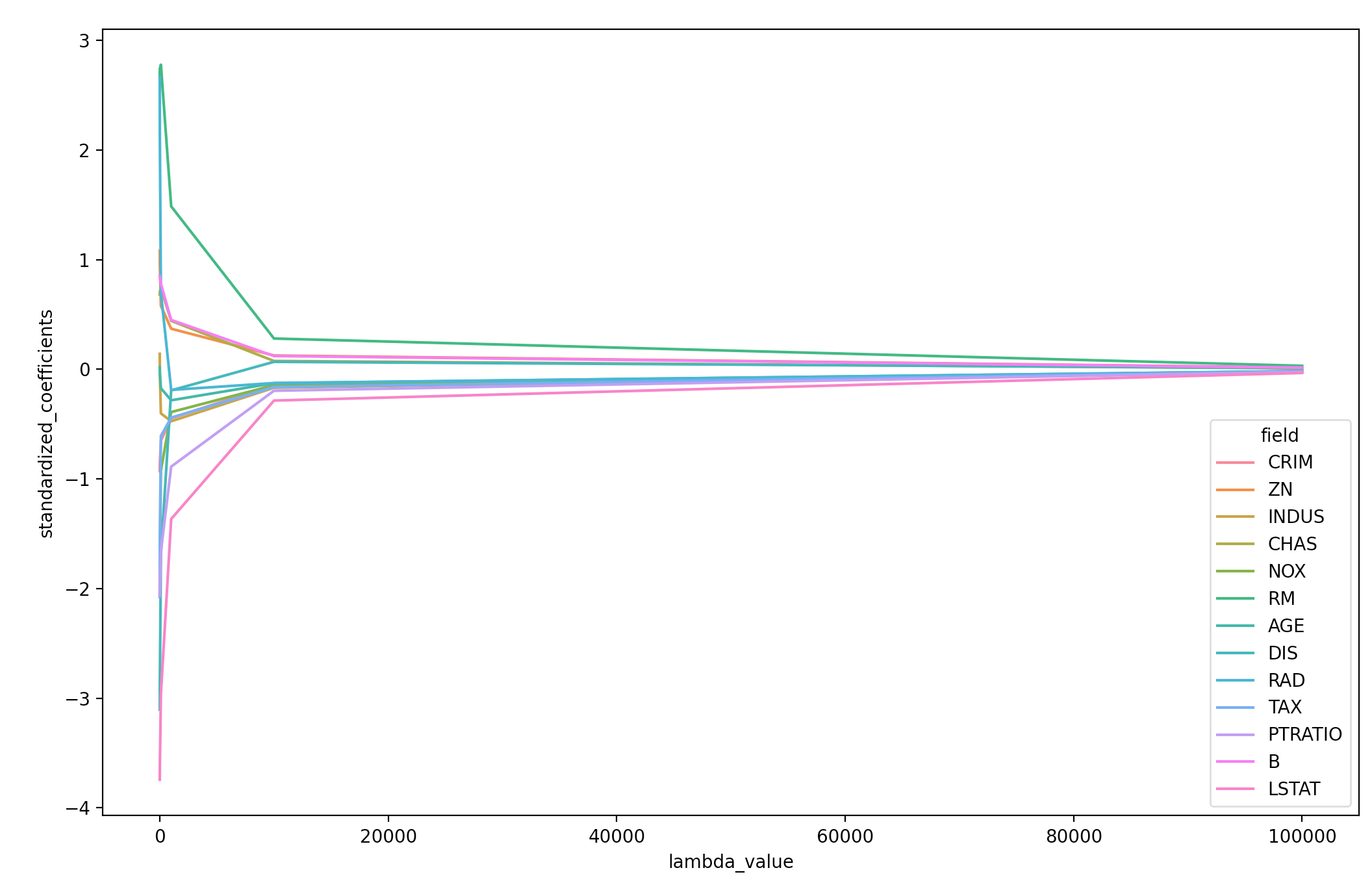
Plotting standardized coefficients as function of $\lambda$
To see how different values of $\lambda$ (alpha) are regularizing the coefficients, we can plot the standardized coefficients as a function of $\lambda$. Below, I’m using lambda and alpha to refer to the same penalty controlling parameter.
import seaborn as sns

# Defining alpha (lambda) values (powers of 10, from 0.00001 to 1000000)
alphas = np.arange(-5, 6)

# Initiating list to hold results
coefficients_list = []

# For each value of alpha, performing ridge regression and storing coefficients
for alpha in 10.0 ** alphas:
    ridge_reg = Ridge(alpha=alpha)
    ridge_reg.fit(X, y)
    coefficients_df = pd.DataFrame(ridge_reg.coef_).T
    coefficients_list.append(coefficients_df)

# Organizing coefficients DataFrame for plotting
coefficients = \
    (pd.concat(coefficients_list)
     .rename(columns=pd.Series(load_boston().feature_names))
     .assign(lambda_value=10.0 ** alphas)
     .set_index("lambda_value")
     .unstack()
     .reset_index()
     .rename(columns={"level_0": "field",
                      0: "standardized_coefficients"})
     .loc[:, ["lambda_value", "field", "standardized_coefficients"]])

# Viewing DataFrame
coefficients

    lambda_value  field  standardized_coefficients
0         0.00001   CRIM                  -0.928146
1         0.00010   CRIM                  -0.928145
2         0.00100   CRIM                  -0.928138
3         0.01000   CRIM                  -0.928061
4         0.10000   CRIM                  -0.927301
..            ...    ...                        ...
138      10.00000  LSTAT                  -3.623942
139     100.00000  LSTAT                  -2.961415
140    1000.00000  LSTAT                  -1.365649
141   10000.00000  LSTAT                  -0.285220
142  100000.00000  LSTAT                  -0.033575

# Plotting standardized coefficients as function of lambda
sns.lineplot(data=coefficients,
             x="lambda_value",
             y="standardized_coefficients",
             hue="field")
The lasso
The scikit-learn API provides parallel functions for performing the lasso instead of ridge regression. For example, we can also use GridSearchCV to determine an optimal alpha value for the lasso.
from sklearn.linear_model import Lasso

# Initializing Lasso and GridSearchCV estimators
lasso = Lasso()
grid_search_lasso = GridSearchCV(estimator=lasso, param_grid=param_grid)

# Fitting grid search object
grid_search_lasso.fit(X, y)

# Results
grid_search_lasso.best_params_     # best alpha=0.1
grid_search_lasso.best_score_      # highest mean 5-fold cross-validated test score (corresponds where alpha=0.1)
grid_search_lasso.score(X, y)      # training score of best model, refit on all folds
Lasso with statsmodels’ OLS.fit_regularized
Lastly, we can also perform ridge regression and the lasso using the statsmodels package. To do this, we’ll need to use the OLS.fit_regularized method and set method="elastic_net". Then, if we set the L1_wt parameter to 0 we can perform ridge regression, and by setting this parameter to 1 we can perform the lasso. Setting L1_wt somewhere between 0 and 1 will perform elastic net regularization, which will be the topic of a future post.
import statsmodels.api as sm

# L1_wt = 1 --> lasso, L1_wt = 0 --> ridge
sm_lasso = sm.OLS(endog=y, exog=sm.add_constant(X))
result = sm_lasso.fit_regularized(method="elastic_net", alpha=0.1, L1_wt=1)
result.params  # viewing standardized coefficients when alpha=0.1