Regularization is a method of fitting a model containing all predictors $p$ that regularize the coefficient estimates towards zero. Also known as constraining or shrinking the model’s coefficient estimates, regularization can significantly reduce the model’s variance and thus improve test error estimates and model performance. The two most commonly used regularization methods are ridge regression and the lasso.
In the below post, I’ll provide an overview of both of these methods. In a future post, I’ll explore using cross-validation to hyperparameter tuning, and will provide working examples of these methods using both Python’s scikit-learn and statsmodels packages.
The structure of this post was influenced by the sixth chapter of An Introduction to Statistical Learning: with Applications in R by Gareth James, Daniela Witten, Trevor Hastie, and Robert Tibshirani.
Ridge regression
Ridge regression can be viewed as an extension of the least squares fitting procedure. The least squares fitting procedure estimates the coefficients $\beta_0, \beta_1, … \beta_p$ as the values that minimize
\[\begin{aligned} RSS = \sum_{i=1}^{n} (y_i - \hat{\beta_0} - \sum_{j=1}^{p} \beta_j x_{ij})^2. \end{aligned}\]In contrast, ridge regression estimates the coefficients by minimizing a similar, but different quantity. In particular, the ridge regression coefficient estimates $\hat{\beta}^R$ are the values that minimize
\[\begin{aligned} \sum_{i=1}^{n} (y_i - \hat{\beta_0} - \sum_{j=1}^{p} \beta_j x_{ij})^2 + \lambda \sum_{j=1}^{p} \beta_j^2 = RSS + \lambda \sum_{j=1}^{p} \beta_j^2 \end{aligned}\]where $\lambda \geq 0$ is a tuning parameter commonly selected using cross-validation. The second term $\lambda \sum_{j=1}^{p} \beta_j^2$ is known as a shrinkage penalty and has the effect of shrinking the estimates $\hat{\beta_0}, \hat{\beta_1}, … \hat{\beta_p}$ towards zero. When $\lambda = 0$, the penalty term has no effect and ridge regression will produce the same coefficient estimates as the least squares estimates. However, as $\lambda \to \inf$, the ridge regression coefficient estimates will approach zero.
Outside the statistical literature, ridge regression is known as Tikhonov regularization (and less commonly Tikhonov–Phillips regularization), after the Russian and Soviet mathematician and geophysicist Andrey Nikolayevich Tikhonov.
 |
|---|
| Source: Gareth James, Daniela Witten, Trevor Hastie, Robert Tibshirani. An Introduction to Statistical Learning: with Applications in R. New York: Springer, 2013. |
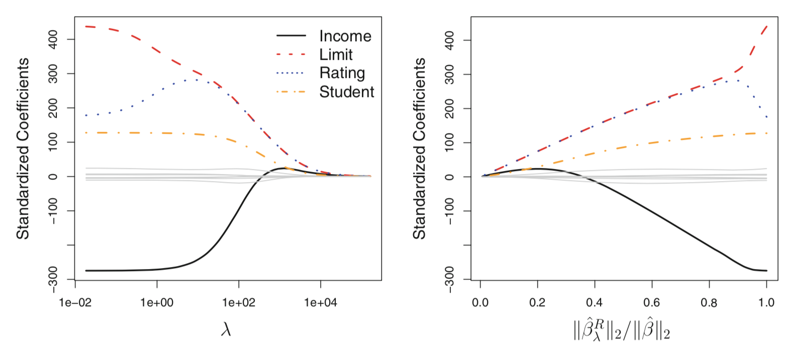
The figure above shows ridge regression performed on the Credit data set (available via the ISLR R package). The left plot shows the standardized coefficients as a function of $\lambda$, while the right plot shows the same coefficients as a function of the $l_2$ $norm$ of the ridge regression coefficient estimates over the $l_2$ $norm$ of the least squares coefficient estimates. From the image, we can see that the Income, Limit, Rating and Student variable approach zero as $\lambda$ increases, while the other variables (dulled out in gray) maintain values near zero for all values of $\lambda$ shown.
Standardizing predictor variables
Note, the ridge regression coefficient estimates are influenced by the scale of the predictor variables. As such, it is best to apply ridge regression after all predictor variables have been scaled such that they each have a mean of zero and a standard deviation of one. While, it is not necessary to also standardize the response variable - and it can make model interpretation slightly more challenging - it does not affect model accuracy.
Improvements over least squares
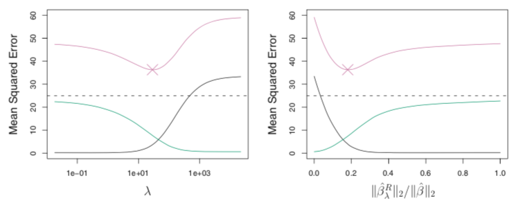
Ridge regression tends to perform better than least squares fitting. This advantage is rooted in the bias-variance trade-off. As $\lambda$ increases, the flexibility of the ridge regression fit decreases, leading to decreased variance but increased bias. This is illustrated in the figure below, where the squared bias is show in black, variance in green, and test mean squared error (MSE) in purple for the ridge regression predictions on a simulated dataset. As $\lambda$ increases, the shrinkage of the ridge regression coefficients towards zero leads to a reduction in the variance of the predictions, at the expense of a slight increase in bias. The test MSE, which is a function of the variance plus squared bias, decreases and then rapidly increases. A minimum value of the test MSE is obtained at approximately $\lambda = 30$.
 |
|---|
| Source: Gareth James, Daniela Witten, Trevor Hastie, Robert Tibshirani. An Introduction to Statistical Learning: with Applications in R. New York: Springer, 2013. |
Furthermore, in situations where the relationship between the response and the predictors is close to linear, the least squares estimates will have low bias but may have high variance. This is especially true if the number of variables $p$ is almost as large as the number of observations $n$. In both of these situations, ridge regression will tend to outperform least squares.
In addition, when $p$ > $n$, the least squares coefficient estimates do not have a unique solution, whereas ridge regression can still be performed.
Ridge regression is also computational advantageous over methods like best subset selection, which requires searching through $2^p$ models.
The lasso
Although ridge regression can perform well, it does have one obvious disadvantage. The method will always include all $p$ predictors in the final model. While the penalty $\lambda \sum_{j=1}^{p} \beta_j^2$ will shrink coefficients towards zero, it will not set any of them exactly to zero (unless $\lambda = \inf$). This may not be a problem for prediction accuracy, but can make model interpretability (and management) challenging when $p$ is large.
The lasso is an alternative to ridge regression that overcomes this disadvantage. The lasso, which was originally an abbreviation for least absolute shrinkage and selection operator, was rediscovered and popularized in the statistical context by Robert Tibshirani in 1996. The lasso coefficients, $\hat{\beta}_{\lambda}^L$, minimize the quantity
\[\begin{aligned} \sum_{i=1}^{n} (y_i - \hat{\beta_0} - \sum_{j=1}^{p} \beta_j x_{ij})^2 + \lambda \sum_{j=1}^{p} |\beta_j| = RSS + \lambda \sum_{j=1}^{p} |\beta_j|. \end{aligned}\]Notice ridge regression and the lasso solve similar optimization problems. The only difference is the $\beta_j^2$ in the ridge regression penalty has been replaced by $|\beta_j|$ in the lasso penalty. The lasso uses an $l_1$ penalty instead of an $l_2$. The $l_1$ norm of a coefficient vector $\beta$ is given by $\Vert\beta\Vert_1 = \sum\vert\beta_j\vert$.
Due to the $l_1$ penalty, the lasso performs coefficient shrinkage but also has the effect of forcing some of the coefficient estimates to be exactly equal to zero when $\lambda$ is sufficiently large. Hence, the lasso performs variable selection, and produces models that are much easier to interpret than those produced by ridge regression. As in ridge regression, cross-validation is often used to select an optimal value of $\lambda$.
 |
|---|
| Source: Gareth James, Daniela Witten, Trevor Hastie, Robert Tibshirani. An Introduction to Statistical Learning: with Applications in R. New York: Springer, 2013. |
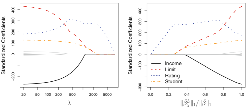
In the above figure, we see the standardized coefficient estimates produced from the lasso on the same Credit data set described above. We see that as $\lambda$ increases, the coefficient estimates for various predictor variables are each forced to zero.
Standardizing predictor variables
Note, that similar to ridge regression, the lasso should be preformed on standardized predictor variables that have been scaled such that they each have a mean of zero and a standard deviation of one.
The variable selection property of the lasso
The lasso and ridge regression coefficient estimates can be shown to solve the problems
\[\begin{aligned} \text{minimize} \{RSS\} \text{ subject to } \sum_{j=1}^{p} |\beta_j| \leq s \end{aligned}\]and
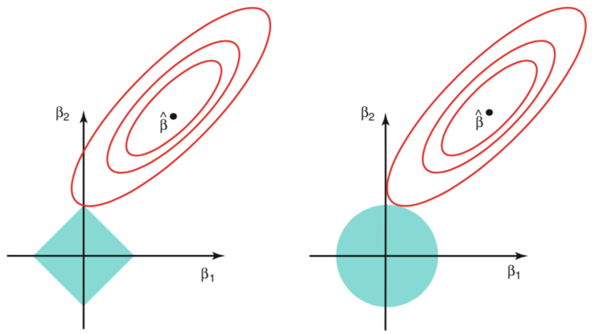
\[\begin{aligned} \text{minimize} \{RSS\} \text{ subject to } \sum_{j=1}^{p} \beta_j^2 \leq s \end{aligned}\]respectively. When $p=2$, the lasso coefficient estimates have the smallest RSS out of all points that lie within the diamond defined by $\lvert \beta_1 \rvert + \lvert \beta_2 \rvert \leq s$. Similar, the ridge regression estimates have the smallest RSS out of all points that lie within the circle defined by $\beta_1^2 + \beta_2^2 \leq s$. This is illustrated in the below figure showing the contours of the errors and constraint functions for the lasso (left) and ridge regression (right). The solid blue areas are the constraint regions $\lvert \beta_1 \rvert + \lvert \beta_2 \rvert \leq s$ and $\beta_1^2 + \beta_2^2 \leq s$, while the red ellipses are the contours of the RSS produced from different model fits. The least squares solution is marked as $\hat{\beta}$.
 |
|---|
| Source: Gareth James, Daniela Witten, Trevor Hastie, Robert Tibshirani. An Introduction to Statistical Learning: with Applications in R. New York: Springer, 2013. |
Because the lasso and ridge regression minimize the RSS subject to their respective constraint functions, the RSS contour line for the lasso will tend to fall on a corner of the diamond, while the RSS contour line for ridge regression will rarely fall directly on an axis intercept. Thus, the lasso has the affect of forcing coefficient estimates to zero, while ridge regression does not.
For $p > 2$, the ideas depicted in the above figure still hold. However, the lasso’s constraint region becomes a polytope, while ridge regression’s constraint region becomes a hypersphere.
Comparing the lasso and ridge regression
While the lasso has the advantage of performing variable selection over ridge regression (and thus producing a simpler and more interpretable model), it is not always clear which method leads to better prediction accuracy.
In general, we can expect the lasso to perform better when a relatively small number of predictors are related to the response. In contrast, we can expect ridge regression to perform better when a relatively large number of the predictors are related to the response. However, in practice, it is rarely known which predictors are related to the response a priori. Thus, a technique such as cross-validation should be used to determine which approach is better on a particular data set. Note, when performing hyperparameter tuning and model evaluation simultaneously, a nested cross-validation procedure should be used.