The bootstrap is a widely used resampling technique first introduced by Bradley Efron in 1979 commonly used to quantify the uncertainty associated with a given estimator or statistical learning method. The bootstrap can be applied to many problems and methods, and is commonly used to estimate the standard errors of the coefficients estimated from regression model fits, or the distribution of $R^2$ values from those fits.
Using bootstrap resampling, we can estimate the uncertainty - or variability - associated with a given method by taking repeated samples from a dataset with replacement and applying the method. For example, to estimate the uncertainly of a coefficient estimate $\hat{\beta_1}$ from a linear regression fit, we take $n$ repeated samples with replacement from our dataset and train our linear regression model $n$ times and record each value $\hat{\beta}_1^{\ast 1}, \ldots, \hat{\beta}_1^{\ast n}$. With enough resampling - typically 1000 or 10,000 - we can plot the distribution of these bootstrapped estimates $\hat{\beta}_1^{\ast 1}, \ldots, \hat{\beta}_1^{\ast n}$. Then, we can use the resulting distribution to quantify the variability of this estimate by calculating useful summary statistics, such as standard errors and confidence intervals. Often, this distribution will approach the Gaussian distribution.
The power of the bootstrap lies in the ability to take repeated samples of the dataset, instead of collecting a new dataset each time. Also, in contrast to standard error estimates typically reported with statistical software that rely on algebraic methods and underlying assumptions, bootstrapped standard error estimates are more accurate as they are calculated computationally. For example, the common standard error estimate for a linear regression fit is dependent upon an unknown parameter $\sigma_2$ that is estimated using the residual sum of squares values. Bootstrapped standard error estimates do not rely on these assumptions and unknown parameters, so they are likely to produce more accurate results.
There are quite a few varieties of the bootstrap, including bootstrap resampling procedures appropriate for time series data. The particular variety of bootstrapping discussed in this post is case resampling, and is likely the most commonly used in practice.
Calculating bootstrapped estimates using scikit-learn’s resample
Unlike in R, which has the boot package to perform bootstrap resampling, I was not able to find any similar robust Python package. I did find a few packages on PyPI for bootstrap resampling in Python, but they all seemed underdeveloped and not commonly used.
However, thankful, scikit-learn does provide a resample function that can be used to perform bootstrap resampling. resample specifically resamples a dataset n_samples times, with the default option to sample with replacement. Therefore, we can use this function in our own loop to perform bootstrap resampling.
Bootstrapped standard error estimates & confidence intervals
For this example, we’ll make use of the common Boston housing dataset. For this first working example, we’ll only concern ourselves with two predictor fields to keep it simple.
import pandas as pd
from sklearn.datasets import load_boston

# Loading boston dataset
boston = load_boston()

# Selecting just two fields and renaming
X = (pd.DataFrame(boston.data, columns=boston.feature_names)
     .loc[:, ["RM", "AGE"]]
     .rename(columns=dict(RM="mean_rooms_per_dwelling",
                          AGE="prop_built_prior_1940")))

y = pd.DataFrame(boston.target, columns=["median_value"])

data = pd.concat(objs=[X, y], axis=1)
Now that our data is organized, let’s construct a for-loop that will train n_iterations linear regression models to our data using bootstrapped resampling. We’ll record the intercept and coefficient terms, as well the $R^2$ values in a DataFrame for inference.
Note, any data preparation or preprocessing of the data must occur within the for-loop and not before. Otherwise, we risk data leakage. Also, it is common to resample the same number of samples as the original dataset. For very large datasets or computationally inefficient processes this is not always required and a percentage of the data can used instead during each iteration.
from sklearn.linear_model import LinearRegression
from sklearn.utils import resample

# Defining number of iterations for bootstrap resample
n_iterations = 1000

# Initializing estimator
lin_reg = LinearRegression()

# Initializing DataFrame, to hold bootstrapped statistics
bootstrapped_stats = pd.DataFrame()

# Each loop iteration is a single bootstrap resample and model fit
for i in range(n_iterations):

    # Sampling n_samples from data, with replacement, as train
    # Defining test to be all observations not in train
    train = resample(data, replace=True, n_samples=len(data))
    test = data[~data.index.isin(train.index)]

    X_train = train.loc[:, ["mean_rooms_per_dwelling", "prop_built_prior_1940"]]
    y_train = train.loc[:, ["median_value"]]

    X_test = test.loc[:, ["mean_rooms_per_dwelling", "prop_built_prior_1940"]]
    y_test = test.loc[:, ["median_value"]]

    # Fitting linear regression model
    lin_reg.fit(X_train, y_train)

    # Storing stats in DataFrame, and concatenating with stats
    intercept = lin_reg.intercept_
    beta_mean_rooms_per_dwelling = lin_reg.coef_.ravel()[0]
    beta_prop_built_prior_1940 = lin_reg.coef_.ravel()[1]
    r_squared = lin_reg.score(X_test, y_test)

    bootstrapped_stats_i = pd.DataFrame(data=dict(
        intercept=intercept,
        beta_mean_rooms_per_dwelling=beta_mean_rooms_per_dwelling,
        beta_prop_built_prior_1940=beta_prop_built_prior_1940,
        r_squared=r_squared
    ))

    bootstrapped_stats = pd.concat(objs=[bootstrapped_stats,
                                         bootstrapped_stats_i])
In the above code, we took 1000 samples of our training data, fit 1000 linear regression models, and calculated 1000 $R^2$ values and recorded 1000 intercept and coefficient estimates.
>>> bootstrapped_stats

    intercept  beta_mean_rooms_per_dwelling  beta_prop_built_prior_1940  r_squared
0  -23.368142                      8.208489                   -0.085221   0.489404
0  -29.051630                      8.920175                   -0.063330   0.448506
0  -30.699820                      9.309012                   -0.080105   0.508171
0  -23.654573                      8.006092                   -0.060957   0.546636
0  -20.861677                      7.702751                   -0.072565   0.586873
..        ...                           ...                         ...        ...
0  -25.539613                      8.418104                   -0.070129   0.604587
0  -12.140724                      6.366914                   -0.089853   0.529767
0  -16.641207                      7.126756                   -0.080550   0.523440
0  -29.418797                      9.081140                   -0.077730   0.497529
0  -24.967460                      8.503919                   -0.088081   0.471693

[1000 rows x 4 columns]
Next, let’s plot this estimates. We’ll plot a separate histogram for each statistic to get an idea of the distribution of each.
import seaborn as sns
import matplotlib.pyplot as plt

# Plotting histograms
fig, axes = plt.subplots(2, 2, figsize=(7, 7))
sns.histplot(bootstrapped_stats["intercept"], color="royalblue", ax=axes[0, 0], kde=True)
sns.histplot(bootstrapped_stats["beta_mean_rooms_per_dwelling"], color="olive", ax=axes[0, 1], kde=True)
sns.histplot(bootstrapped_stats["beta_prop_built_prior_1940"], color="gold", ax=axes[1, 0], kde=True)
sns.histplot(bootstrapped_stats["r_squared"], color="teal", ax=axes[1, 1], kde=True)
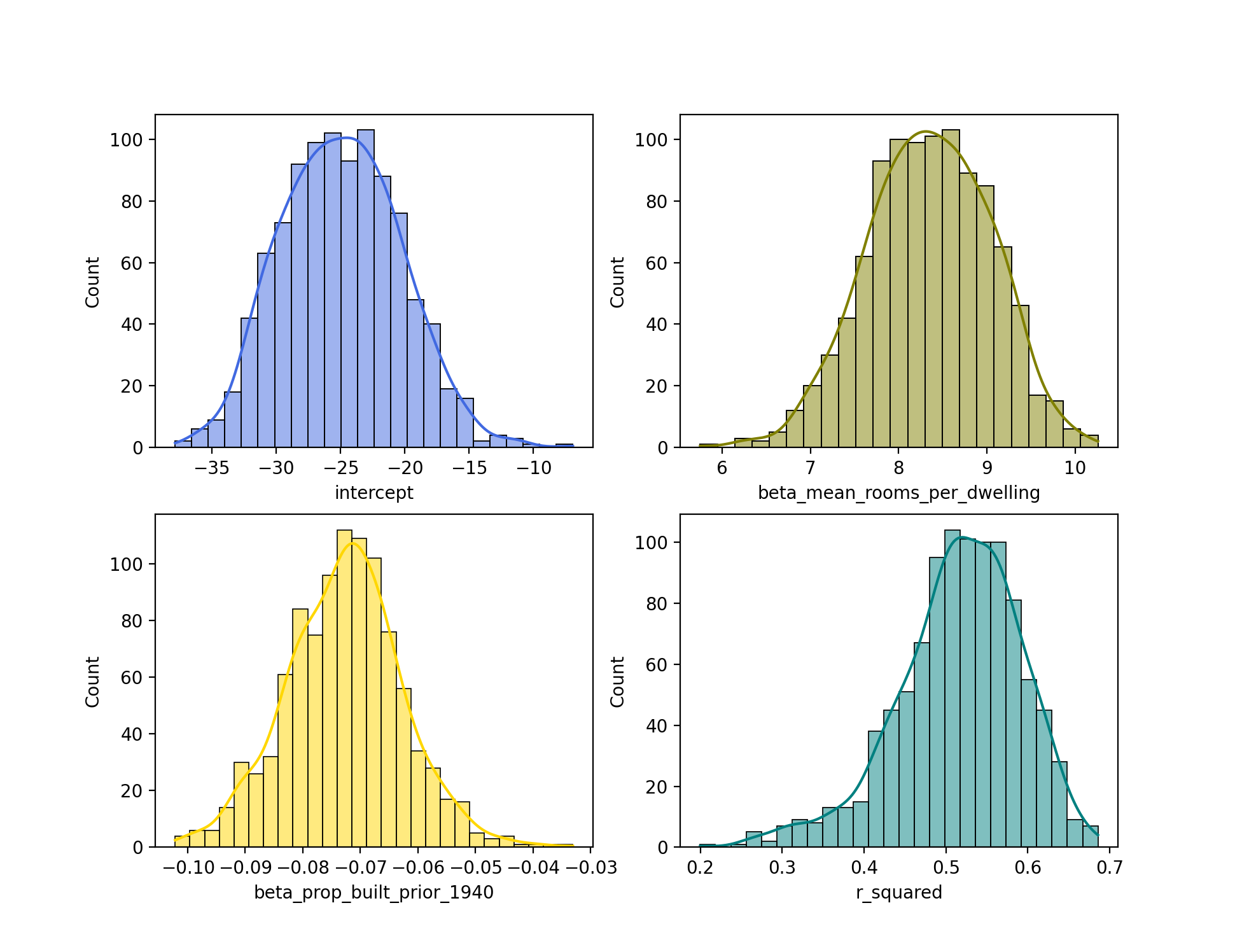
From the histograms, we can see that each of the distributions approximates the normal distribution. Interestingly, the distribution for r_squared is slightly left skewed.
We can perform some basic inference of these estimates as well. Let’s estimate the standard error of the beta_mean_rooms_per_dwelling statistic using scipy’s tstd - or trimmed standard deviation - function. Note, it might be tempting here to use scipy’s sem - or standard error of mean/measurement - function instead. Because we already have our distribution of 1000 estimates, the standard deviation of this distribution is actually what we want, and the standard error is actually an estimated standard deviation for a sampling distribution.
The standard deviation is a measure of variability, being used here to estimate the variability of the population of possible bootstrapped statistics. If instead, I was interested in how the mean of these bootstrapped statistics (not the statistics themselves) varied across many bootstrap resampling procedures, I would calculate the standard error.
>>> import scipy.stats as st

>>> st.tstd(bootstrapped_stats["beta_mean_rooms_per_dwelling"])
0.6971573554752794
scipy’s tstd function has the default parameter ddof=1. Here, ddof stands for delta degrees of freedom. A ddof of 1 indicates the degrees of freedom should be equal to $n - 1$. Notably, NumPy’s default ddof value is 0, equivalent to $n$ degrees of freedom. The below two function calls produce the same results.
import numpy as np

st.tstd(bootstrapped_stats["beta_mean_rooms_per_dwelling"])
np.std(bootstrapped_stats["beta_mean_rooms_per_dwelling"], ddof=1)
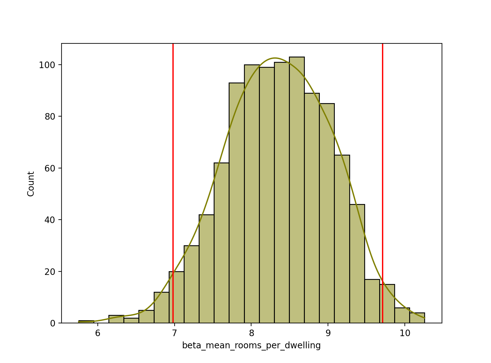
Lastly, let’s calculate a 95% confidence interval for our beta_mean_rooms_per_dwelling estimates, and plot the upper and lower bounds as vertical red lines on the histogram. Note, we can use the normal approximation here (via st.norm.interval) because of our large sample size of 1000 bootstrap estimates. If we instead had a small number of samples below 30 or 50, it would be more appropriate to use the t-distribution instead, via st.t.interval.
ci = st.norm.interval(alpha=0.95,
                      loc=np.mean(bootstrapped_stats["beta_mean_rooms_per_dwelling"]),    # mean
                      scale=st.tstd(bootstrapped_stats["beta_mean_rooms_per_dwelling"]))  # standard deviation

# Plotting confidence interval on histogram
sns.histplot(bootstrapped_stats["beta_mean_rooms_per_dwelling"], color="olive", kde=True)
plt.axvline(x=ci[0], color="red")
plt.axvline(x=ci[1], color="red")
Bootstrapped $R^2$ estimates for lasso regression
As a simple extension, we can also use Lasso regression instead of linear regression. Below, I show similar code as above that calculates 1000 bootstrapped $R^2$ estimates.
from sklearn.linear_model import Lasso

# Instead of np.hstack, could have used np.concatenate([boston.data, boston.target.reshape(-1,1)], axis=1)
data_all = pd.DataFrame(
    data=np.hstack((boston.data, boston.target.reshape(-1, 1))),
    columns=np.concatenate([boston.feature_names, ["median_value"]])
)

# Defining number of iterations for bootstrap resample
n_iterations = 1000

# Initializing estimator
lasso = Lasso()

# Initializing DataFrame, to hold bootstrapped statistics
bootstrapped_lasso_r2 = pd.Series()

# Each loop iteration is a single bootstrap resample and model fit
for i in range(n_iterations):

    # Sampling n_samples from data, with replacement, as train
    # Defining test to be all observations not in train
    train = resample(data_all, replace=True, n_samples=len(data_all))
    test = data_all[~data_all.index.isin(train.index)]

    X_train = train.iloc[:, 0:-1]
    y_train = train.iloc[:, -1]

    X_test = test.iloc[:, 0:-1]
    y_test = test.iloc[:, -1]

    # Fitting linear regression model
    lasso.fit(X_train, y_train)

    # Storing stats in DataFrame, and concatenating with stats
    r_squared = lasso.score(X_test, y_test)

    bootstrapped_lasso_r2_i = pd.Series(data=r_squared)

    bootstrapped_lasso_r2 = pd.concat(objs=[bootstrapped_lasso_r2,
                                            bootstrapped_lasso_r2_i])
scikit-learn’s BaggingRegressor
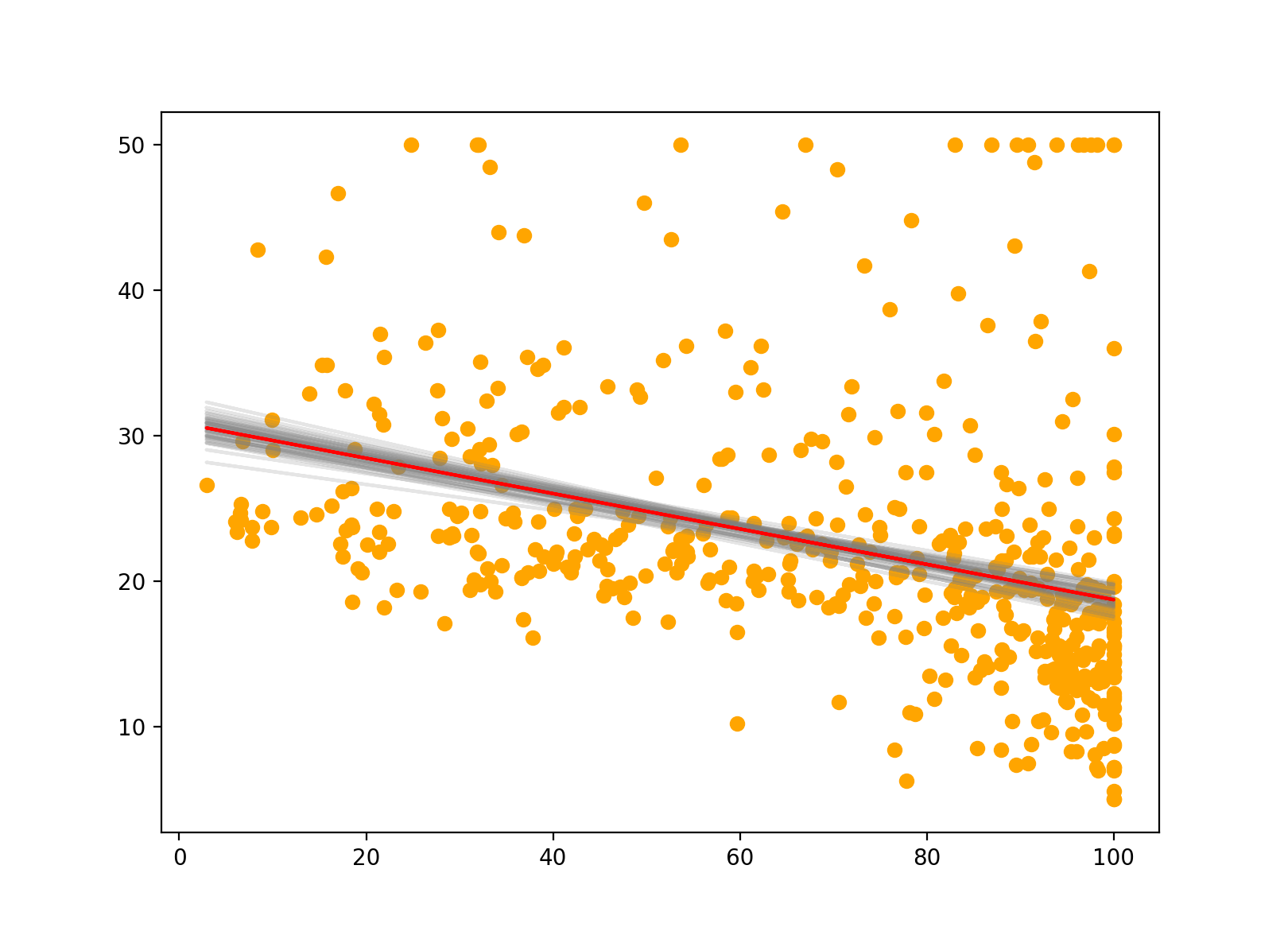
Lastly, we can also use scikit-learn’s BaggingRegression to fit multiple bootstrapped regression models to our data. This is similar to the above, and we can easily see the variability of the different models in our plot. The red line indicates the bagged prediction line. In a future post, I’ll explore bagging in much greater detail.
from sklearn.ensemble import BaggingRegressor

X = data[["prop_built_prior_1940"]]
y = data[["median_value"]]

n_estimators = 50

# Initializing estimator
model = BaggingRegressor(LinearRegression(),
                         n_estimators=n_estimators,
                         bootstrap=True)

# Fitting 50 bootstrapped models
model.fit(X, y)

plt.figure(figsize=(12, 8))

# Plotting each model
for m in model.estimators_:
    plt.plot(X, m.predict(X), color="grey", alpha=0.2, zorder=1)

# Plotting data
plt.scatter(X, y, color="orange")

# Bagged model prediction
plt.plot(X, model.predict(X), color="red")