In this post, I’ll be exploring quadratic discriminant analysis. I’ll compare and contrast this method with linear discriminant analysis, and work through an example using scikit-learn and the slimmed down Titanic dataset from one of my prior posts on logistic regression.
The structure of this post was influenced by the fourth chapter of An Introduction to Statistical Learning: with Applications in R by Gareth James, Daniela Witten, Trevor Hastie, and Robert Tibshirani.
Quadratic discriminant analysis
As discussed in earlier posts, linear discriminant analysis (LDA) assumes that the observations are drawn from a multivariate Gaussian distribution with a class specific mean vector, and a covariance matrix $\Sigma$ that is common across all $K$ classes. In contrast, quadratic discriminant analysis (QDA) uses a different approach. While both LDA and QDA assume the observations are drawn from a multivariate Gaussian distribution with a class specific mean vector, QDA assumes that each class $k$ has its own covariance matrix $\Sigma_k$. Thus, QDA assumes an observation from the $k$th class is of the form $X \sim N(\mu_k, \Sigma_k)$.
Both LDA and QDA classify results by using estimates of the underlying Gaussian distribution the observations are drawn from in Bayes’ theorem, and then classifying an observation to the class for which the posterior probability $Pr(Y = k \vert X = x)$ is greatest. In contrast to LDA however, under the alternative assumptions of QDA, the Bayes classifier is equivalent to assigning an observation $X = x$ to the class for which
\[\begin{aligned} \delta_k(x) &= -\frac{1}{2}(x-\mu_k)^T \sum_{k}^{-1}(X-\mu_k) - \frac{1}{2} \text{log } \vert \sum_{k} \vert + \text{log } \pi_k \\ &= -\frac{1}{2}x^T \sum_{k}^{-1}x + x^T\sum_{k}^{-1}\mu_k - \frac{1}{2}\mu_k^T\sum_{k}^{-1}\mu_k - \frac{1}{2} \text{log } \vert \sum_{k} \vert + \text{log } \pi_k \end{aligned}\]is largest.
So, the QDA classifier takes estimates for $\Sigma_k$, $\mu_k$, and $\pi_k$ and plugs them into the above equation to calculate $\delta_k$. Then, the observation is assigned to the class for which $\delta_k$ is largest. Unlike in linear discriminant analysis, $x$ appears as a quadratic function in the above equation. This is why QDA is named as it is.
When to prefer LDA or QDA
When would we prefer LDA over QDA, or vice-versa? In general, LDA tends to perform better than QDA when there are relatively few training observations. In contrast, QDA is recommended when the training set is very large, or if the assumption of a common covariance matrix for all $K$ classes is clearly not reasonable.
These recommendations have to do with the bias-variance trade off. When there are $p$ predictors, estimating a single covariance matrix requires estimating $p(p+1)/2$ parameters. However, QDA estimates a separate covariance matrix for each class, for a total of $Kp(p+1)/2$ parameters.
Consequently, LDA is less flexible classifier than QDA, and thus has significantly lower variance. That is, when trained on new training sets, the model will tend to produce similar results (i.e., a lower variance of the predicted values). However, there is a trade-off here. If the assumption that all $K$ classes share a common covariance matrix is untrue, then LDA can suffer from high bias. That is, the model will be strongly effected by the characteristics of the training set, and will not be able to capture the true relations between the predictor and response variables (i.e., the model will be biased towards a particular training set).
Thus, LDA prefers better when there are relatively few training observations because reducing variance is crucial. In contrast, QDA is preferred when the training set is very large, as the variance of the classifier is not a major concern.
 |
|---|
| Source: Gareth James, Daniela Witten, Trevor Hastie, Robert Tibshirani. An Introduction to Statistical Learning: with Applications in R. New York: Springer, 2013. |
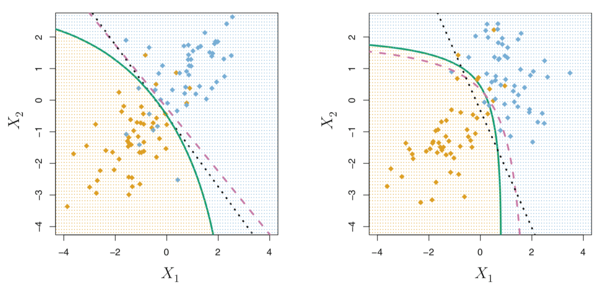
The above image shows the performance of LDA and QDA in two scenarios. In the left-hand panel, the classes are Gaussian distributed and have a common correlation of 0.7 between $X_1$ and $X_2$. In the right-hand panel, the classes are still Gaussian distributed, but the orange class has a correlation of 0.7 between the variables, while the blue class has a correlation of -0.7 between the variables. Thus, in the right-hand panel, $\Sigma_{\text{orange}} \neq \Sigma_{\text{blue}}$
In the left-hand panel, we see that the black dotted LDA decision boundary approximates the purple dashed Bayes decision boundary quite well. The green solid QDA decision boundary does not perform as well because it suffers from higher variance without a corresponding decrease in bias. However, in the right-hand panel, we see the Bayes decision boundary is now quadratic, so QDA more accurately approximates this boundary than does LDA.
A scikit-learn example
Next, let’s explore using scikit-learn to perform quadratic discriminant analysis on our titanic dataset.
import pandas as pd
from sklearn.discriminant_analysis import QuadraticDiscriminantAnalysis

# Assigning X and y
X = titanic[["age", "fare"]]
y = titanic["survived"]

# Fitting model
qda = QuadraticDiscriminantAnalysis()
qda.fit(X, y)
qda.score(X, y)  # 0.647
After fitting our model, the correct classification score for QDA is approximately 0.647. We can also view the model’s precision, recall, $F_1$ score, and accuracy using scikit-learn’s classification_report function.
>>> print(classification_report(y_true=y, y_pred=qda.predict(X)))

              precision    recall  f1-score   support
           0       0.64      0.94      0.76       424
           1       0.72      0.21      0.33       290

    accuracy                           0.65       714
   macro avg       0.68      0.58      0.55       714
weighted avg       0.67      0.65      0.59       714
For comparison purposes, let’s perform a linear discriminant analysis on the same predictor and response variables.
from sklearn.discriminant_analysis import LinearDiscriminantAnalysis

lda = LinearDiscriminantAnalysis()
lda.fit(X, y)
lda.score(X, y)  # 0.647
Interestingly, our LDA model has a correct classification rate that is exactly equal that of our earlier QDA model. However, the precision, recall, and $F_1$ score values have changed slightly.
>>> print(classification_report(y_true=y, y_pred=lda.predict(X)))

           0       0.64      0.94      0.76       424
           1       0.71      0.22      0.34       290

    accuracy                           0.65       714
   macro avg       0.67      0.58      0.55       714
weighted avg       0.67      0.65      0.59       714
Finally, let’s compare our two models by plotting their ROC curves and comparing the area under the curve for each.
import matplotlib.pyplot as plt

from sklearn.metrics import plot_roc_curve

roc_qda = plot_roc_curve(estimator=qda, X=X, y=y)
roc_log_reg = plot_roc_curve(estimator=lda, X=X, y=y, ax=roc_qda.ax_)
plt.title("ROC Curve Comparison")
plt.show()
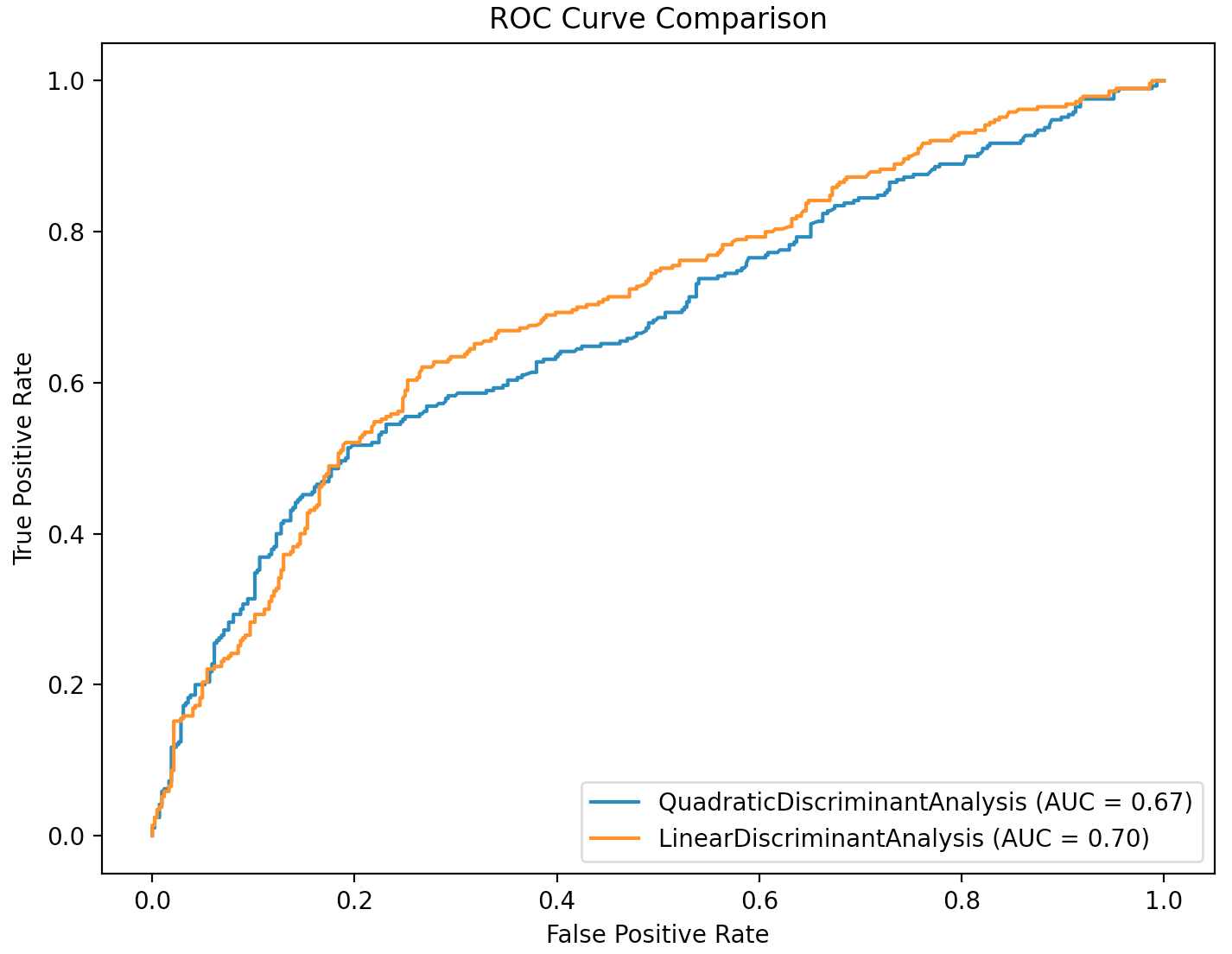
From above, we see that the AUC value for our LDA model is slightly higher than that of our QDA model, indicating the LDA model is a better performing classifier, at least on our training data.