This post is the second in a series on the logistic regression model. In this post, I’ll work through an example using the well known Titanic dataset, scikit-learn and statsmodels. I’ll discuss one-hot encoding, create a 3D logistic regression plot using Plotly, and demonstrate multiclass logistic regression with scikit-learn.
Titanic dataset
In this example, I’ll be using the Kaggle’s Titanic training dataset
The Titanic dataset is available from many sources. In this example, I’ll be using Kaggle’s Titanic training dataset. You can download the data manually, or use Kaggle’s command line interface. After reading in the data as titanic, let’s take a quick peek at it.
>>> titanic.info()
<class 'pandas.core.frame.DataFrame'>
RangeIndex: 891 entries, 0 to 890
Data columns (total 12 columns):
 #   Column       Non-Null Count  Dtype
---  ------       --------------  -----
 0   PassengerId  891 non-null    int64
 1   Survived     891 non-null    int64
 2   Pclass       891 non-null    int64
 3   Name         891 non-null    object
 4   Sex          891 non-null    object
 5   Age          714 non-null    float64
 6   SibSp        891 non-null    int64
 7   Parch        891 non-null    int64
 8   Ticket       891 non-null    object
 9   Fare         891 non-null    float64
 10  Cabin        204 non-null    object
 11  Embarked     889 non-null    object
dtypes: float64(2), int64(5), object(5)
memory usage: 83.7+ KB

>>> titanic.head()
   PassengerId  Survived  Pclass  ...     Fare Cabin  Embarked
0            1         0       3  ...   7.2500   NaN         S
1            2         1       1  ...  71.2833   C85         C
2            3         1       3  ...   7.9250   NaN         S
3            4         1       1  ...  53.1000  C123         S
4            5         0       3  ...   8.0500   NaN         S
[5 rows x 12 columns]
I find snake_case column names much easier to working with, so let’s do some quick clean up. I decided to explore the janitor library for this, and made use of the clean_names() function. And since we’re only interested in a subset of fields here, let’s go ahead and select just those fields to keep via pandas loc method.
import janitor
import pandas as pd

titanic = (janitor
          .clean_names(titanic)
          .loc[:, ["sex", "age", "fare", "pclass", "survived"]]
          .rename(columns={"pclass": "ticket_class"}))
Now that our data is cleaned up, let’s take a quick look around to see if we have any missing values.
>>> titanic.isna().sum()
sex               0
age             177
fare              0
ticket_class      0
survived          0
dtype: int64
We can see that there are 177 missing age values. In a future post, I’ll explore methods of imputing missing values, and when and why imputing is appropriate. But for this working example, let’s just remove these observations from our dataset.
titanic = titanic.query("age.notna()").reset_index()
Lastly, since at first we’ll be attempted to classify whether a passenger survived or not, let’s look at the frequency of survived.
titanic["survived"].value_counts()
0    424
1    290
Out of the 714 passengers in our current dataset, only 290 survived, or about 41%. In many classification problems, we might be interested in equaling out these binary classes to produce a better predictive model. A variety of upsampling and downsampling techniques exist for this, which I’ll explore in future posts. For this example however, we’ll just take the class frequencies as it, but keep in mind that better results may be possible with more robust methods.
Simple logistic regression
To keep it simple at first, let’s start out with a logistic regression model with only a single predictor, age.
X = titanic[["age"]]
y = titanic["survived"]
scikit-learn
Let’s use scikit-learn’s LogisticRegression() first to train our model. Note, by default, LogisticRegresson() preforms variable regularization. We can disable this by passing penalty="none" when we initialize the classifier.
from sklearn.linear_model import LogisticRegression

# Initializing classifier
log_reg = LogisticRegression(penalty="none")

# Fitting model
log_reg.fit(X=X, y=y)

log_reg.score(X, y)
The score method here provides the correct classification rate. For this particular model, 59.4% of the observations were correctly classified.
We can verify the correct classification rate is being provided by manually calculating it.
y_hat = log_reg.predict(y.to_numpy().reshape(-1, 1))
correct_class_rate = np.sum(y == y_hat) / len(y)

sklearn_score = log_reg.score(X, y)

>>> np.equal(sklearn_score, correct_class_rate)
True
With a little more investigation into the results of our model, we can see that this model doesn’t have very much predictive potential. Let’s look at the unique predicted values of our model
import numpy as np

np.unique(y_hat)
This yields a single unique predicted value, 0. This indicates our model is predicting that every passenger will not survive. By plotting our model, we can learn some more information.
import seaborn as sns

sns.regplot(x="age", y="survived", data=titanic, logistic=True)
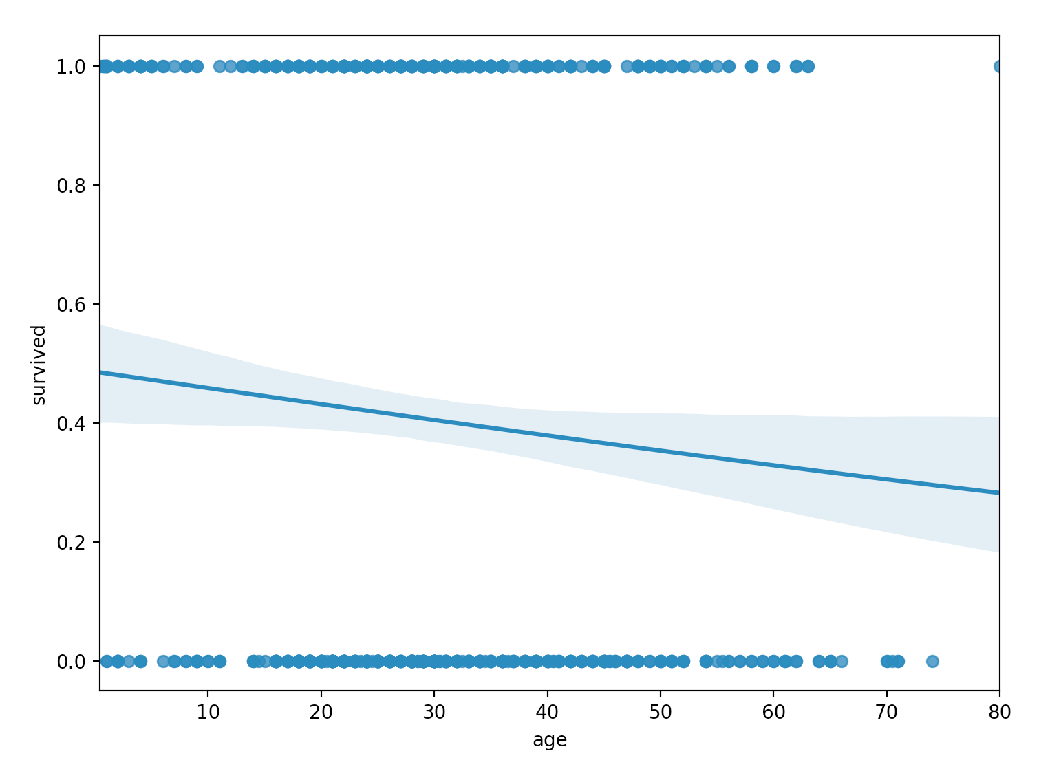
From the plot, we don’t see the characteristic $S$-shaped sigmoid function of the logistic regression model. Instead, we do see a sigmoid function, but it more-or-less appears equivalent to a linear function for the particular domain of our data. Clearly, age alone is not explaining our survived response variable well.
Before adding new predictors to our model, let’s perform the same regression as above using the statsmodels library.
statsmodels: Logit()
statsmodels provides two functions for performing logistic regression. The first is the Logit() function provided in the discrete_model module. The second is the GLM() function. We’ll explore the Logit() function first.
import statsmodels.api as sm

from statsmodels.discrete.discrete_model import Logit

model = Logit(endog=y, exog=sm.add_constant(X))
result = model.fit()
Remember, in statsmodels, an intercept term is not included by default. So to perform the same regression as scikit-learn, we’ll have to add an intercept via sm.add_constant().
As usual with statsmodels, a wealth of summary information is provided by the summary() method.
result.summary()
<class 'statsmodels.iolib.summary.Summary'>
"""
                           Logit Regression Results
==============================================================================
Dep. Variable:               survived   No. Observations:                  714
Model:                          Logit   Df Residuals:                      712
Method:                           MLE   Df Model:                            1
Date:                Sat, 30 Jan 2021   Pseudo R-squ.:                0.004445
Time:                        10:12:45   Log-Likelihood:                -480.11
converged:                       True   LL-Null:                       -482.26
Covariance Type:            nonrobust   LLR p-value:                   0.03839
==============================================================================
                 coef    std err          z      P>|z|      [0.025      0.975]
------------------------------------------------------------------------------
const         -0.0567      0.174     -0.327      0.744      -0.397       0.283
age           -0.0110      0.005     -2.057      0.040      -0.021      -0.001
==============================================================================
"""
Worth mentioning here is the pseudo $R^2$ summary statistic, labeled Pseudo R-squ. The pseudo $R^2$ statistic is a measure of how well a logistic regression model explains the response variable, akin to a linear regression model’s $R^2$ statistic. A variety of pseudo $R^2$ statistics have been proposed, and statsmodels reports McFadden’s pseudo $R^2$, published in 1974. While McFadden’s pseudo $R^2$ statistic can take values between 0 and 1, a value in the range of 0.2 to 0.4 is considered an excellent fit. Not surprisingly, our value of 0.004445 is quite low, confirming our model does not fit the data well.
One useful feature about the statsmodels implementation is that probabilities, not just classes, are reported. We can get the probability that an observations survived by using the predict() method.
>>> probs = model.predict(params=result.params)

# First 10 probabilities
>>> probs[:10]
array([0.42606613, 0.38382723, 0.41537876, 0.39163506, 0.39163506, 0.34327126,
       0.48034749, 0.4127189 , 0.44763968, 0.47487681])
statsmodels: GLM()
statsmodels also provides the GLM() function, which when the family parameter is set to Binomial(), produces the same results as the above two methods.
from statsmodels.genmod.families.family import Binomial

model = sm.GLM(endog=y, exog=sm.add_constant(X), family=Binomial())
result = model.fit()
result.summary()
Multiple logistic regression
Next, let’s explore using multiple predictors to improve our model fit. In particular, we’ll include sex and fare in addition to age. Because sex is a categorical feature, we’ll need to encode it via scikit-learn’s OneHotEncoder. In a future post, I’ll explore creating scikit-learn Pipelines and making use of the new ColumnTransformer. However, for this demonstration, I’ll keep it simple and perform this encoding in discrete steps
from sklearn.preprocessing import OneHotEncoder

# Initializing one-hot encoder
# Forcing dense matrix to be returned, dropping first encoded column
encoder = OneHotEncoder(sparse=False, drop="first")

# Encoding categorical field
X_categorical = titanic[["sex"]]
X_categorical = encoder.fit_transform(X_categorical)

# Numeric fields
X_numeric = titanic[["age", "fare"]]

# Concatenating categorical and numeric fields together
X = np.concatenate((X_categorical, X_numeric), axis=1)

# Fitting model
log_reg = LogisticRegression(penalty="none")
log_reg.fit(X=X, y=y)
log_reg.score(X, y)
This correct classification rate for this model is 0.777, which is a sizable improvement over the earlier value of 0.594.
Using statsmodels’ GLM(), let’s do some statistical inference to see if all of the predictor variables are significant.
model = sm.GLM(endog=y, exog=sm.add_constant(X), family=Binomial())
result = model.fit()

>>>result.summary()
<class 'statsmodels.iolib.summary.Summary'>
"""
                 Generalized Linear Model Regression Results
==============================================================================
Dep. Variable:               survived   No. Observations:                  714
Model:                            GLM   Df Residuals:                      710
Model Family:                Binomial   Df Model:                            3
Link Function:                  logit   Scale:                          1.0000
Method:                          IRLS   Log-Likelihood:                -358.04
Date:                Sat, 30 Jan 2021   Deviance:                       716.07
Time:                        10:51:29   Pearson chi2:                     701.
No. Iterations:                     5
Covariance Type:            nonrobust
==============================================================================
                 coef    std err          z      P>|z|      [0.025      0.975]
------------------------------------------------------------------------------
const          0.9348      0.239      3.910      0.000       0.466       1.403
x1            -2.3476      0.190    -12.359      0.000      -2.720      -1.975
x2            -0.0106      0.006     -1.627      0.104      -0.023       0.002
x3             0.0128      0.003      4.738      0.000       0.007       0.018
==============================================================================
"""
From the summary table, we see that the x2 variable, or age, is not statistically significant.
3D Plot
As a last exploration of this model, let’s drop the age variable and create a three-dimensional plot of our multiple logistic regression model. We’ll make use of the Plotly library for this.
import plotly.express as px
import plotly.graph_objects as go

# Define mash size for prediction surface
mesh_size = .02

# Removing age field because not significant
# obj=1 refers to age column
X_sex_fare = np.delete(X, obj=1, axis=1)

# Fitting model
log_reg.fit(X=X_sex_fare, y=y)

# Define x and y ranges
# Note: y here refers to y-dimension, not response variable
x_min, x_max = X_sex_fare[:, 0].min(), X_sex_fare[:, 0].max()
y_min, y_max = X_sex_fare[:, 1].min(), X_sex_fare[:, 1].max()
xrange = np.arange(x_min, x_max, mesh_size)
yrange = np.arange(y_min, y_max, mesh_size)
xx, yy = np.meshgrid(xrange, yrange)

# Get predictions for all values of x and y ranges
pred = log_reg.predict(X=np.c_[xx.ravel(), yy.ravel()])

# Reshape predictions to match mesh shape
pred = pred.reshape(xx.shape)

# Plotting
fig = px.scatter_3d(titanic,
                    x='sex',
                    y='fare',
                    z='survived',
                    labels=dict(sex="Sex (1 if male, 0 if female)",
                                fare="Ticket Fare",
                                survived="Survived"))
fig.update_traces(marker=dict(size=5))
fig.add_traces(go.Surface(x=xrange, y=yrange, z=pred, name='pred_surface'))
fig.show()

While our prediction surface is a little jerky, this plot does provide a useful interpretation of our model. We see that women are more likely to survive, and as are men with ticket fares of over 150.
It is important to note here that this prediction surface does not actually represent the model. In particular, since sex is binary, it doesn’t make sense for an observation to have a sex value of 0.5. A more accurate representation would be two logistic regression functions on either end of the visible plane - one when sex == 0 and another when sex == 1. However, I think the plane does provide a good representation of the relationship between these two functions.
Multiclass logistic regression
As a last exploration into the logistic regression model, I’ll explore a multiclass logistic regression.
For this example, I’ll train a model to predict the ticket_class variable using sex, age, and survived As we’ve already seen using fare, we can likely expect ticket_class to be associated with survived.
Similar to above, we’ll first encode sex.
# Initializing one-hot encoder
# Forcing dense matrix to be returned, dropping first encoded column
encoder = OneHotEncoder(sparse=False, drop="first")

# Encoding categorical field
X_categorical = titanic[["sex"]]
X_categorical = encoder.fit_transform(X_categorical)

# Numeric fields
X_numeric = titanic[["age", "survived"]]

# Concatenating categorical and numeric fields together
X = np.concatenate((X_categorical, X_numeric), axis=1)

y = titanic[["ticket_class"]].to_numpy().ravel()
We’ll then train the model using scikit-learn’s LogisticRegression(). This function natively handles multiclass logistic regression. Unless specified otherwise, it will using a one-vs-rest scheme for prediction. Under the hood, this scheme will train an individual model for each class present in the data. Because ticket_class can take three possible values 1, 2, or 3, we can expect three logistic regression models to be trained.
The one-vs-rest (sometimes called one-vs-all) scheme can be contrasted with the one-vs-one scheme. The one-vs-one scheme splits the dataset into individual datasets containing only two classes. For example, using ticket_class field, the one-vs-one method would create individual models for the following ticket_class pairs:
ticket_class1 vsticket_class2ticket_class1 vsticket_class3ticket_class2 vsticket_class3
To perform prediction, each observation is run through it’s associated models, and the class label with the most predictions is the overall prediction.
In addition, scikit-learn does provide the OneVsRestClassifier and the OneVsOneClassifier as well, which are commonly used with support vector classifiers.
# Uses a one-vs-rest scheme by default
log_reg = LogisticRegression(penalty="none")
log_reg.fit(X=X, y=y)
The correct classification rate for our model is about 0.599, and we can view the first 10 predicted classes using the predict() method.
>>> log_reg.score(X, y)
0.5994397759103641

>>> log_reg.predict(X)[:10]
array([3, 1, 1, 1, 3, 1, 3, 1, 3, 3])