I recently read through Chip Huyen’s Designing Machine Learning Systems, first published in 2022. I found it a highly useful overview of a rapidly evolving field. As I expected from her other writings, Chip provided clear explanations while straddling the line nicely between technical depth and summarization. Machine learning engineering and machine learning operations contain a vast ecosystem of solutions, tools, and ever-evolving methods. Summarizing the relevant concepts is not an easy task to do.
In no particular order, here are some insights I found helpful. Some of these are tiny tidbits of knowledge, while others are lengthy topics that I’ll attempt to summarize in a few paragraphs. I intentionally didn’t include topics I was already familiar with, such as transfer learning or experiment tracking.
- Batch processing is a special case of stream processing
- Consider creating an in-house labeling team
- Weak supervision
- Semi-supervision
- Active learning
- Prioritize long-tail accuracy for class imbalance regression tasks
- Consider the Precision-Recall Curve for class imbalance classification tasks
- Data-level resampling methods
- Algorithm-level resampling methods
- Hashing Trick for encoding categorical features
Batch processing is a special case of stream processing
In hindsight, this is a bit obvious, but I didn’t make the connection until coming across it in Designing Machine Learning Systems. In stream processing, data is processed in real-time as it becomes available. The data arrives continuously, often at varying rates and speeds. If we instead store the data as it comes in, and then process it in discrete chunks, we have batch processing.
Of course, batch processing and stream processing each have their pros and cons, and for many machine learning applications, you might need features computed from both.
Consider creating an in-house labeling team
If your organization or problem could significantly benefit from more labeled data, and can’t get that labeled data from elsewhere, and techniques such as semi-supervised learning aren’t sufficient, creating an in-house data labeling team could have incredible valuable.
Of course, not every organization can devote so many resources to just data labeling. But if your organization can, it’s worth considering.
Apparently, Tesla maintains a team of over 1,000 people devoted to data labeling.
Weak supervision
Weak supervision refers to the notion of using heuristics to label data. Often, these heuristics are developed by working with subject matter experts who have deep domain knowledge.
Weak supervision is a simple and powerful approach, but is not perfect. Often the labels obtained by weak supervision are noisy - sometimes too noisy to be useful as your solution matures. Even so, weak supervision can be helpful to explore the effectiveness of ML for a particular problem without having to invest in hand labeling up-front.
Semi-supervision
In contrast to weak supervision, where heuristics are used to obtain noisy labels, semi-supervision leverages structural assumptions in your data to generate new labels. Semi-supervision does require a small set of initial labels.
There are many semi-supervised learning methods. Self-training is a classic method, where you start by training a model on your existing set of labeled data and use this model to make predictions on unlabeled samples. You then add the predictions with high enough probability scores to your training set and train a new model on this larger training set. This process is repeated until you’re satisfied with your model performance.
Another collection of semi-supervised learning methods involves using a clustering or ${k}$-nearest neighbors algorithm to discover samples that belong to the same cluster. Samples that do not have a label are assigned the label of the other samples in that cluster.
A third semi-supervision method is the perturbation-based method, where small perturbations are applied to training samples to obtain new training samples. These perturbations can be applied to the samples themselves (e.g., adding white noise to images), or their representations (e.g., adding small random values to embeddings of words). The perturbed samples are assigned the same labels as the unperturbed samples. This method is based on the assumption that small perturbations to a sample shouldn’t change it’s label.
In past roles, I’ve worked on multiple cold-start anomaly detection problems. In these settings, unsupervised approaches can be helpful to bootstrap label creation. For example, a clustering algorithm or density-based algorithm such as Local Outlier Factor can be used to first group observations. From here, domain knowledge labels can be assigned to each cluster, and a semi-supervised approach can then be used to improve model performance. If you’re working on a cold-start anomaly detection problem like this and come across anomalies during exploratory data analysis, document the anomalies you find. These anomalies can be grouped and labels can eventually be applied to also kick off a semi-supervised learning solution.
Active learning
Active learning is a method for improving the efficiency of data labels when we have only a small labeled training set. The idea is that we let the model decide which data samples to learn from, and this can improve performance. Instead of randomly hand-labeling samples, we label samples that are most helpful to the model.
In a classification setting, we might hand-label the examples our model is most uncertain about, hoping to improve the model’s decision boundaries. Another approach is called query-by-committee, and it involves using an ensemble of models to vote on which sample to label next. A human then labels the samples that the model committee disagrees on the most. A third approach could be choosing samples to label, which if trained on them, would result in the largest gradient updates or reduce the loss the most.
Prioritize long-tail accuracy for class imbalance regression tasks
Class imbalance is most often discussed in the context of classification tasks - the classic example being rare cancer prediction tasks. But class imbalance can also happen with regression tasks, such as estimating healthcare bills or student absences, where underlying distributions can be quite skewed. In these cases, especially when we care more about accurately predicting values towards the tail of the distribution, we might want to train our models to be better at predicting the 80th or 95th percentile.
In particular, pinball loss can be used to train your model to be better at predicting a particular percentile. This might reduce overall metrics, such as root mean squared error, but that might be a reasonable trade-off for certain problems.
Consider the Precision-Recall Curve for class imbalance classification tasks
The traditional ROC curve focuses only on the positive class and doesn’t show how well your model did on the negative class. Davis and Goadrich suggested instead that we should plot precision against recall. They argue this Precision-Recall Curve, provides a better overall summary of an algorithm’s performance when a task has heavy class imbalance.
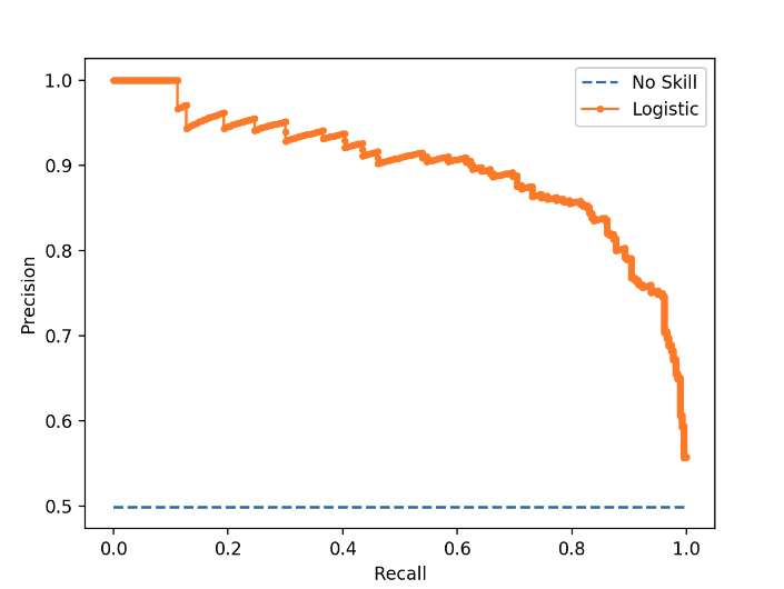 |
|---|
| Source: Machine Learning Mastery |
Data-level resampling methods
For class imbalance problems, Chip shares a variety of strategies to reduce the level of imbalance, so that the model can learn easier. Resampling methods include both oversampling and undersampling. Oversampling refers to adding more observations from the minority classes, while undersampling refers to removing observations of the minority classes. This simplest way to oversample is to randomly make copies of the minority class, while the simplest way to undersample is to randomly remove instances from the majority class.
When undersampling via randomly dropping observations, we risk losing important data that could influence our model learning and performance. When oversampling via simply duplicating existing observations, we risk overfitting to these duplicated observations.
Some more sophisticated data-level resampling methods are below.
Tomek links
Tomek links, developed in 1976 by Ivan Tomek, can be used to find pairs of observations from opposite classes that are close in proximity and remove the sample of the majority class in each pair. This is an undersampling method, ideal for low-dimensional data. Tomek links are available via imbalance learn’s under_sampling.TomekLinks method.
SMOTE
Synthetic minority oversampling technique (SMOTE) is a method of oversampling low-dimensional data. It synthesizes novel samples of the minority class to balance the class distribution.
Two-phase learning
Two-phase learning is an approach that involves training a model in two distinct phases. It’s often used when we have limited available data for the task we care about. In the first phase, we train our model on a task where we have enough available data or that is easier to learn. In the second phase, we fine-tune our pre-trained model on the task we care about. We do this by updating the model’s parameters using a small amount of labeled data.
We can adapt two-phase learning to mitigate the class imbalance problem. We first randomly undersample large classes until each class has ${N}$ observations. We then train our model on this resampled dataset and fine-tune our model on the original dataset.
Dynamic sampling
Dynamic sampling is a strategy published in 2018 by Pouyanfar et al. that oversamples low-performing classes and undersamples high-performing classes during training. Essentially, the method shows the model less of what it has already learned and more of what it has not.
Algorithm-level resampling methods
In contrast to the above data-level resampling methods that attempt to mitigate the class imbalance challenge by altering the training data distribution, algorithm-level methods alter the training algorithm to make it more robust to class imbalances.
Cost-sensitive learning
Rooted in the observation that misclassification of different classes incurs different costs, cost-sensitive learning uses a cost matrix to specify ${C_{ij}}$, or the cost if class ${i}$ is predicted as class ${j}$. For a correct classification, the cost is usually 0. For a misclassification, the cost is hand-defined for that particular case of misclassification.
This method is problematic because the cost matrix has to be manually defined, which can be challenging at scale.
Class-balanced loss
Class-balanced loss is a particular formation of the loss function that penalizes the model for making wrong predictions on minority classes. In its most basic form, we can assign a weight for each class that is inversely proportional to the number of samples in that class, such that rarer samples have higher weights:
\[\begin{aligned} W_i = \frac{\text{total number of training samples}}{\text{number of samples of class } i} \end{aligned}\]The loss incurred by observation ${x}$ of class ${i}$ is shown below, where Loss(${x}$, ${j}$) is the loss when ${x}$ is classified as class ${j}$. Loss(${x}$, ${j}$) could be cross-entropy or any other loss function. ${\theta}$ refers to the model’s parameter set.
\[\begin{aligned} L(x; \theta) = W_i \sum_j P(j|x;\theta)\cdot{}\text{Loss}(x, j) \end{aligned}\]Ensembles for class imbalances
Ensembles of models have been shown in practice to help with the class imbalance problem. However, ensemble methods are typically used for other purposes, such as improving accuracy and reducing overfitting, as opposed to mitigating class imbalances.
Ensembles of models can also be challenging to manage and deploy in production.
Hashing Trick for encoding categorical features
The Hashing Trick is a technique to encode categorical features. It’s particularly useful when you have an unbounded number of possible categorical features in your data, such as school_name or university_department_name. Encoding these values from $0$ to $n-1$ would work until a new school_name or university_department_name was added to your dataset.
A better approach would be to assign the index value of these fields a random value from a pre-determined hash table. This is advantageous because you can determine how large the hashed space is, and a good hashing function will roughly uniformly assign random hashed values to your categorical features.
The Hashing Trick does have one downside: collision. Collision occurs when two categorical features are assigned the same index value. However, Booking.com has shown even extreme collision only marginally affects performance.
➡️ You can find my second post on 11 more takeaways from Designing Machine Learning Systems here.