This post is the first in a series on the linear discriminant analysis method. In this series, I’ll discuss the underlying theory of linear discriminant analysis, as well as applications in Python.
The structure of this post was influenced by the fourth chapter of An Introduction to Statistical Learning: with Applications in R by Gareth James, Daniela Witten, Trevor Hastie, and Robert Tibshirani.
Linear discriminant analysis
In logistic regression, we model $Pr(Y=k \vert X=x)$ using the logistic function. Specifically, we model the conditional distribution of the response $Y$, given the predictors $X$.
In contrast, in discriminant analysis, we use an alternative and less direct approach to estimating these probabilities. Instead of directly modeling $Pr(Y=k \vert X=x)$, we model the distribution of the predictors $X$ separately for each of the response classes of $Y$. We then use Bayes’ theorem to flip these around into estimates for $Pr(Y=k \vert X=x)$. When the distributions of the predictors $X$ are assumed to be normal, linear discriminant analysis takes a form very similar to logistic regression.
If logistic regression and linear discriminant analysis end up taking such similar forms, then why do we need both? There are several key reasons:
-
In the case where the response classes of $Y$ are well-separated, the parameter estimates for the logistic regression model are surprisingly unstable. This causes them to swing and vary, and does not produce an accurate prediction for all cases. Linear discriminant analysis does not suffer from this problem.
-
In the case where n, the sample size, is small and the distribution of the predictors $X$ is approximately normal in each of the response classes, the linear discriminant model is again more stable than the logistic regression model.
-
In the case where we have more than two response classes, linear discriminant analysis is an attractive approach over multiclass logistic regression.
Bayes’ theorem for classification
Next, we’ll explore using Bayes’ theorem for classification. Bayes’ theorem will allow us to perform the “flip” discussed above to determine estimates for $Pr(Y=k \vert X=x)$. I’ll simultaneously introduce the theory and discuss a working example to clarify understanding.
Suppose we wish to classify an observation into one of $K$ classes, where $K \geq 2$. Let $\pi_k$ represent the overall or prior probability that a randomly chosen observation belongs to the $k$th class. Let $f_k(x) \equiv Pr(X=x \vert Y=k)$, where $f_k(x)$ denotes the density function of X for an observation that comes from the $k$th class. Remember, the total area under a density curve is always equal to one, indicating that across multiple values of $x$, the area under $f_k(x)$ is equal to one, for a specific class $k$.
Note, $f_k(x) \equiv Pr(X=x \vert Y=k)$ is technically only true when $X$ is a discrete random variable. For the event where $X$ is continuous, $f_k(x)dx$ corresponds to the probability of $X$ falling in a small region $dx$ around $x$.
Let’s explore an example. Imagine the United States, the United Kingdom and Canada are comparing the times it takes their citizens to run an 800-meter run. The United States provides the times for 200 of their citizens, the United Kingdom provides the times for 300 of their citizens, and Canada provides the times for 100 of their citizens.
Let’s find the prior probability that a random chosen person is from the USA. In notation, this is equivalent to $\pi_{USA}$. Of course, this is just equal to
\[\begin{aligned} \pi_{USA} = \frac{200 \text{ USA citizens}}{600 \text{ total citizens}}. \end{aligned}\]The density function for the USA class, or $f_{USA}(x)$, is a function indicating the probability that a given observation $x$ ran a given 800-meter run in minutes $f(x)$, where $x$ belongs to the USA class. We can imagine that some runners might be very fast and run times below 2 minutes, while some will be slow and run times greater than four minutes. However, most will likely run times between two and a half minutes and three and a half minutes. The probability an America runs under 2 minutes is low, but the probability an American runs between two and four minutes is quite high.
Then Bayes’ theorem states that
\[\begin{aligned} Pr(Y = k \vert X = x) = \frac{\pi_k f_k(x)}{\sum_{l=1}^{K}\pi_l f_l(x)}. \end{aligned}\]Notice, we can use estimates of $\pi_k$ and $f_k(X)$ to compute $p_k(X)$, where $p_k(X) = Pr(Y = k \vert X = x)$. In general, it is straightforward to estimate $\pi_k$ if we have a random sample of observation with responses from the populations. However, estimating the density function $f_k(X)$ can be more challenging, unless we assume some simple forms for these densities.
$p_k(X)$ is referred to as the posterior probability that an observation $X = x$ belongs to the $k$th class.
In our example, let’s calculate the posterior probability that runners with 800-meter times of three minutes are American. Let’s imagine for simplicity that 50 American’s run a time of exactly three minutes, while 10 Britains and 20 Canadians run a time of exactly three minutes. Thus, the posterior probability that an observation $X = 3 \text{ minutes}$ was ran by an American is
\[\begin{aligned} p_{USA}(X=300) = \frac{50\text{ USA Citizens}}{50\text{ USA Citizens} + 10\text{ UK Citizens} + 20\text{ CA Citizens}} = \frac{50}{80} = 0.625. \end{aligned}\]Lastly, the Bayes classifier classifies an observation to the class for which $p_k(X)$ is largest. This classifier has the lowest possible error rate of all classifiers. Therefore, if we can correctly estimate $\pi_k$ and $f_k(X)$, we can develop a classifier that approximates the Bayes classifier. This is the basis for linear discriminant analysis.
Linear Discriminant Analysis with One Predictor
Using the above information, let’s explore linear discriminant analysis for the case where we have one predictor variable. First, we need to obtain an estimate of the density function $f_k(X)$. Once we obtain this estimate, we then estimate $p_k(x)$ and classify an observation $x$ to the class for which $p_k(x)$ is largest.
In order to estimate $f_k(x)$, we’ll assume it has a Gaussian form. In the one-dimensional setting, the normal density takes the form
\[\begin{aligned} f_k(x) = \frac{1}{\sqrt{2\pi}\sigma_k} \text{exp}\big(-\frac{1}{2\sigma_k^2}(x-\mu_k)^2\big), \end{aligned}\]where $\mu_k$ and $\sigma_k^2$ are the mean and variance values of the $k$th class. For now, we will further assume that $\sigma_1^2 = \ldots = \sigma_K^2$, and we will denote this by $\sigma^2$. Using our estimate for $f_k(x)$ above, we can rewrite Bayes’ theorem above as
\[\begin{aligned} p_k(x) = \frac{\pi_k \frac{1}{\sqrt{2\pi}\sigma} \text{exp}\big(-\frac{1}{2\sigma^2}(x-\mu_k)^2\big)}{\sum_{l=1}^{K}\pi_l \frac{1}{\sqrt{2\pi}\sigma} \text{exp}\big(-\frac{1}{2\sigma^2}(x-\mu_l)^2\big)}. \end{aligned}\]By manipulating the above equation, we can show that assigning an observation $X=x$ to the class for which $p_k(x)$ is largest is equivalent to the assigning the observations to the class for which
\[\begin{aligned} \delta_k(x) = x \cdot \frac{\mu_k}{\sigma^2} - \frac{\mu_k^2}{2\sigma^2} +\text{log }(\pi_k) \end{aligned}\]is largest.
 |
|---|
| Source: Gareth James, Daniela Witten, Trevor Hastie, Robert Tibshirani. An Introduction to Statistical Learning: with Applications in R. New York: Springer, 2013. |
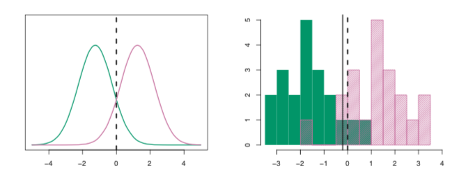
In the above image on the left, two density functions $f_1(x)$ and $f_2(x)$ are shown, representing two distinct classes. In the above image on the right, 20 observations drawn from each class are shown as histograms. Because the data is simulated, the Bayes decision boundary can be calculated, and is shown as the dashed vertical line in each image. In practice, knowing the true Bayes decision boundary is rarely possible. Using the known values of $\mu_1$, $\mu_2$, $\sigma_1$, and $\sigma_2$, $\delta_1(x)$ and $\delta_2(x)$ where calculated for all training values of $x$. The linear discriminant analysis (LDA) decision boundary estimated from the training data is shown as the solid vertical line. Values of $x$ on the left side of the line would be assigned to the green class, while values of $x$ on the right side of the line would be assigned to the purple class. Notice that the LDA decision boundary is close but not exactly equal to the Bayes decision boundary.
Unlike the above example, in practice, we must estimate the parameters $u_1, \ldots, \mu_K, \pi_1, \ldots, \pi_K$, and $\sigma^2$. The LDA method approximates the Bayes classifier using the following estimates for $\pi_k$, $\mu_k$, and $\sigma^2$:
\[\begin{align*} \hat{\mu}_k = \frac{1}{n_k}\sum_{i:y_i=k}x_i \\ \hat{\sigma}^2 = \frac{1}{n-K}\sum_{k=1}^{K}\sum_{i:y_i=k}(x_i - \hat{\mu_k})^2 \\ \hat{\pi}_k = \frac{n_k}{n} \end{align*}\]where $n$ is the total number of training observations, and $n_k$ is the number of training observations in the $k$th class. Here, $\hat{\mu}_k$ is simply the average of all the training observations from the $k$th class, $\hat{\sigma}^2$ can be seen as a weighted average of the sample variances for each of the $K$ classes, and $\hat{\pi}_k$ is the proportion of the training observations that belong to the $k$th class.
Thus, using these estimates, the LDA classifier assigns an observation $X=x$ to the class for which
\[\begin{aligned} \delta_k(x) = x \cdot \frac{\hat{\mu_k}}{\hat{\sigma}^2} - \frac{\hat{\mu}_k^2}{2\hat{\sigma}^2} +\text{log }(\hat{\pi}_k) \end{aligned}\]is largest.
The classifier is referred to as linear because the discriminant functions $\hat{\delta}_k$ are linear functions of $x$.
Linear discriminant analysis with multiple predictors
Next, let’s extend the LDA classifier to the case of multiple predictors. For this, we’ll assume that $X = (X_1, X_2, \ldots, X_p)$ is drawn from a multivariate Gaussian distribution with a class-specific mean vector and a common covariance matrix.
 |
|---|
| Source: Gareth James, Daniela Witten, Trevor Hastie, Robert Tibshirani. An Introduction to Statistical Learning: with Applications in R. New York: Springer, 2013. |
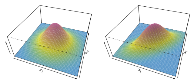
Two multivariate Gaussian density functions are shown above for $p=2$, where $p$ is the number of predictors. In the left image, the two predictors are uncorrelated. In the right image, the two predictors have a correlation of 0.7
To indicate that a $p$-dimensional random variable $X$ has a multivariate Gaussian distribution, we write $X \sim N(\mu, \Sigma)$, where $E(X) = \mu$ is the mean of $X$ and $\text{Cov}(X) = \Sigma$ is the $p \times p$ covariance matrix of $X$. The multivariate Gaussian density is formally defined as
\[\begin{aligned} f(x) = \frac{1}{(2\pi)^{p/2}\vert \Sigma \vert^{1/2}}\text{exp} \big(-\frac{1}{2}(x - \mu)^T \Sigma^{-1} (x-\mu) \big). \end{aligned}\]In the case of multiple predictors, the LDA classifier assumes that the observations in the $k$th class are drawn from a multivariate Gaussian distribution $N(\mu_k, \Sigma)$, where $\mu_k$ is a class-specific mean vector, and $\Sigma$ is a covariance matrix that is common to all $K$ classes. By inserting the above density function for the $k$th class, $f_k(X=x)$, into Bayes’ theorem and performing some manipulation, we can show that the Bayes classifier assigns an observation $X=x$ to the class for which
\[\begin{aligned} \delta_k(x) = x^T \Sigma^{-1} \mu_k - \frac{1}{2} \mu_K^T \Sigma^{-1} \mu_k + \text{log } \pi_k \end{aligned}\]is largest.
As before, we need to estimate the unknown parameters $\mu_1, \ldots, \mu_K, \pi_1, \ldots, \pi_K$, and $\Sigma$. The formulas to do these are similar to those discussed in the previous section. To assign a new observation $X = x$, LDA uses these estimates to calculate $\hat{\delta}_k(x)$, and then classifies the observation to the class for which $\hat{\delta}_k(x)$ is largest.
In a future post, I’ll explore investigating the results of an LDA classifier via calculated statistics such as false positive rates (Type I error, 1 - specificity), true positive rates (sensitivity, recall), precision, as well as ROC curves.