This is the fifth post in a series on the multiple linear regression model. In previous posts, I introduced the theory behind the model, exploring using Python’s scikit-learn and statsmodels libraries, and discussed potential problems with the model, such as collinearity and correlation of the error terms.
In this post, I’ll once again compare scikit-learn and statsmodels, and will explore how to include interaction terms and non-linear relationships in the model. I’ll also discuss nuances and potential problems of the resulting models, and possible areas for improvement using more sophisticated techniques.
Boston housing sataset
I’ll make use of the classic Boston Housing Dataset for this working example. This dataset, originally published by Harrison, D. and Rubinfeld, D.L in 1978 has become one of the more common toy datasets for regression analysis. The dataset contains information on 506 census tracts around the Boston, MA area, and is available via scikit-learn.
from sklearn import datasets

boston = datasets.load_boston()
datasets.load_boston() returns a scikit-learn bunch object. We can view information about the dataset via the DESCR attribute.
>>> print(boston.DESCR)
.. _boston_dataset:
Boston house prices dataset
---------------------------
**Data Set Characteristics:**
    :Number of Instances: 506
    :Number of Attributes: 13 numeric/categorical predictive. Median Value (attribute 14) is usually the target.
    :Attribute Information (in order):
        - CRIM     per capita crime rate by town
        - ZN       proportion of residential land zoned for lots over 25,000 sq.ft.
        - INDUS    proportion of non-retail business acres per town
        - CHAS     Charles River dummy variable (= 1 if tract bounds river; 0 otherwise)
        - NOX      nitric oxides concentration (parts per 10 million)
        - RM       average number of rooms per dwelling
        - AGE      proportion of owner-occupied units built prior to 1940
        - DIS      weighted distances to five Boston employment centres
        - RAD      index of accessibility to radial highways
        - TAX      full-value property-tax rate per $10,000
        - PTRATIO  pupil-teacher ratio by town
        - B        1000(Bk - 0.63)^2 where Bk is the proportion of blacks by town
        - LSTAT    % lower status of the population
        - MEDV     Median value of owner-occupied homes in $1000's
Instead of using the return_X_y parameter that returns two numpy arrays, I’ll create a pandas DataFrame for ease of use below.
import pandas as pd

X_df = pd.DataFrame(boston.data, columns=boston.feature_names)
y_df = pd.DataFrame(boston.target, columns=["MEDV"])
boston_df = pd.concat(objs=[X_df, y_df], axis=1)
Qualitative predictors & dummy encoding
Most of the predictors in the Boston housing dataset are quantitative. The CHAS variable however, indicating if the census tract is bounded by the Charles River or not is qualitative and has been pre-encoded as 0 or 1.
I’ll make use of the encoded CHAS variable in the models below. However, for demonstration and to familiarize myself with the procedure, below I create a new categorical field crime_label and encode it via scikit-learn’s OneHotEncoder() class.
from sklearn.preprocessing import OneHotEncoder

# Creating crime_label field
boston_df = \
    (boston_df
     .assign(
        crime_label=pd.cut(boston_df["CRIM"],
                           bins=3,
                           labels=["low_crime", "medium_crime", "high_crime"]))
    )

# Converting crime_label field to NumPy array
crime_labels_ndarray = boston_df["crime_label"].to_numpy().reshape(-1, 1)

# Defining encoder
encoder = OneHotEncoder()

# Fitting encoder on array, and transforming
crime_labels_encoded = encoder.fit_transform(crime_labels_ndarray)

# Converting encoded array to DataFrame
crime_labels_df = pd.DataFrame(data=crime_labels_encoded.toarray(),
                               columns=encoder.get_feature_names())

# Concatenating with boston_df
boston_df = pd.concat(objs=[boston_df, crime_labels_df], axis=1)
boston_df now contains three addition fields, indicating the encoded values of crime_label.
>>> boston_df.head()
      CRIM    ZN  INDUS  ...  x0_high_crime  x0_low_crime  x0_medium_crime
0  0.00632  18.0   2.31  ...            0.0           1.0              0.0
1  0.02731   0.0   7.07  ...            0.0           1.0              0.0
2  0.02729   0.0   7.07  ...            0.0           1.0              0.0
3  0.03237   0.0   2.18  ...            0.0           1.0              0.0
4  0.06905   0.0   2.18  ...            0.0           1.0              0.0
Note, it is common in some use cases to drop an encoded column, as this column can be inferred explicitly from the other columns. This can be accomplished by passing drop="first to OneHotEncoder().
encoder = OneHotEncoder(drop="first")
It is also possible to achieve a similar result using pandas get_dummies().
pd.get_dummies(boston_df["crime_label"], drop_first=True)
Removing the additive assumption: Interaction terms
Next, I’ll explore relaxing the additive assumption of the multiple linear regression model. In particular, I’ll train a model on MEDV versus ZN, CHAS and RM. For ease of use, user readability, and statistical inference results, I’ll use the formula interface provided by statsmodels first, and then scikit-learn’s interface further below.
Let’s first train a model with no interaction terms, for comparison purposes.
>>> import statsmodels.formula.api as smf
>>> model = smf.ols(formula="MEDV ~ ZN + CHAS + RM", data=boston_df)
>>> result = model.fit()
>>> result.summary()
<class 'statsmodels.iolib.summary.Summary'>
"""
                            OLS Regression Results
==============================================================================
Dep. Variable:                   MEDV   R-squared:                       0.522
Model:                            OLS   Adj. R-squared:                  0.519
Method:                 Least Squares   F-statistic:                     182.5
Date:                Mon, 25 Jan 2021   Prob (F-statistic):           5.18e-80
Time:                        08:35:33   Log-Likelihood:                -1653.6
No. Observations:                 506   AIC:                             3315.
Df Residuals:                     502   BIC:                             3332.
Df Model:                           3
Covariance Type:            nonrobust
==============================================================================
                 coef    std err          t      P>|t|      [0.025      0.975]
------------------------------------------------------------------------------
Intercept    -30.4697      2.654    -11.480      0.000     -35.684     -25.255
ZN             0.0666      0.013      5.182      0.000       0.041       0.092
CHAS           4.5212      1.126      4.017      0.000       2.310       6.733
RM             8.2635      0.428     19.313      0.000       7.423       9.104
==============================================================================
Omnibus:                      116.852   Durbin-Watson:                   0.757
Prob(Omnibus):                  0.000   Jarque-Bera (JB):              675.350
Skew:                           0.866   Prob(JB):                    2.24e-147
Kurtosis:                       8.388   Cond. No.                         248.
==============================================================================
Notes:
[1] Standard Errors assume that the covariance matrix of the errors is correctly specified.
"""
From the model summary, we see that all the variables are significant. Let’s take a look at the residual plot to see if any patterns standout.
import seaborn as sns

y = boston_df["MEDV"]
y_hat = result.predict()
resid = y - y_hat

sns.scatterplot(x=y_hat, y=resid).set(xlabel="Predicted Value",
                                      ylabel="Residual")
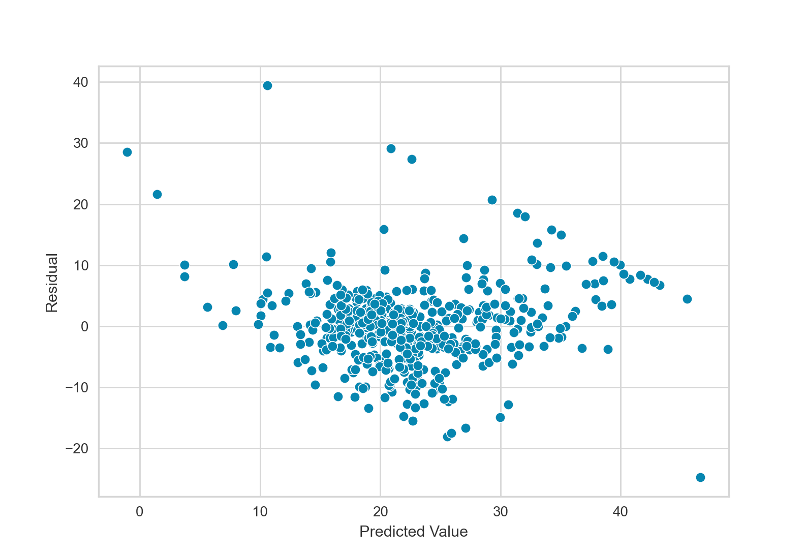
This residual plot does appear to have a pattern. Response values in the middle of the plot tend to be overestimates (negative residuals), while response values on the left and right of the plot tend to be underestimates (positive residuals).
I’ll explore adding some interaction terms here to the model to see if the fit is improved. In the formula notation, a colon : is used to indicate an interaction term. I could have also used an asterisk * to indicate an interaction term as well as the main effects.
>>> model = smf.ols(formula="MEDV ~ ZN + CHAS + RM + ZN:CHAS + CHAS:RM + ZN:RM", data=boston_df)
>>> result = model.fit()
>>> result.summary()
<class 'statsmodels.iolib.summary.Summary'>
"""
                            OLS Regression Results
==============================================================================
Dep. Variable:                   MEDV   R-squared:                       0.537
Model:                            OLS   Adj. R-squared:                  0.531
Method:                 Least Squares   F-statistic:                     96.35
Date:                Mon, 25 Jan 2021   Prob (F-statistic):           3.88e-80
Time:                        19:02:17   Log-Likelihood:                -1645.6
No. Observations:                 506   AIC:                             3305.
Df Residuals:                     499   BIC:                             3335.
Df Model:                           6
Covariance Type:            nonrobust
==============================================================================
                 coef    std err          t      P>|t|      [0.025      0.975]
------------------------------------------------------------------------------
Intercept    -26.4011      2.980     -8.860      0.000     -32.256     -20.547
ZN            -0.4591      0.132     -3.467      0.001      -0.719      -0.199
CHAS           5.0981      9.048      0.563      0.573     -12.679      22.875
RM             7.6154      0.480     15.870      0.000       6.673       8.558
ZN:CHAS       -0.0320      0.065     -0.490      0.625      -0.161       0.097
CHAS:RM       -0.0813      1.411     -0.058      0.954      -2.853       2.690
ZN:RM          0.0783      0.020      3.978      0.000       0.040       0.117
==============================================================================
Omnibus:                      116.146   Durbin-Watson:                   0.715
Prob(Omnibus):                  0.000   Jarque-Bera (JB):              651.824
Skew:                           0.869   Prob(JB):                    2.87e-142
Kurtosis:                       8.282   Cond. No.                     5.88e+03
==============================================================================
Notes:
[1] Standard Errors assume that the covariance matrix of the errors is correctly specified.
[2] The condition number is large, 5.88e+03. This might indicate that there are
strong multicollinearity or other numerical problems.
"""
The above model fit is slightly improved with a $R^2$ statistic of 0.537, compared to 0.522 for the model with no interaction terms. The pattern in the residual plot (not shown) is also slightly improved, but these improvements are minor.
Worth noting as well is that the terms CHAS, ZN:CHAS and CHAS:RM are all no longer significant. Thus, I’ll drop these terms from all subsequent models.
Instead of using the formula interface, I could have also fit these models using the endog and exog parameters of the statsmodels OLS() function. Below is an example, fitting the same model as above, but removing the terms that are no longer significant.
import statsmodels.api as sm

X = boston_df[["ZN", "RM"]].assign(ZN_RM=boston_df["ZN"] * boston_df["RM"])
X = sm.add_constant(X)
y = boston_df["MEDV"]

model = sm.OLS(endog=y, exog=X)
result = model.fit()
result.summary()
In below examples, I’ll show how polynomial regression models can be fit via the scikit-learn API.
Removing the linear assumption: Polynomial regression
In addition to relaxing the additive assumption of the linear regression model, next I’ll explore relaxing the linear assumption by including some polynomial terms.
Using the PolynomialFeatures() class from scikit-learn’s preprocessing module, I’ll train a polynomial regression model. Note, the degree parameter of PolynomialFeatures() has a default value of 2 indicating each predictor and each interaction term up to the power of 2 will be included in the model,
from sklearn import linear_model
from sklearn.preprocessing import PolynomialFeatures

poly = PolynomialFeatures()
X = poly.fit_transform(X=boston_df[["ZN", "RM"]])
y = boston_df["MEDV"]

model = linear_model.LinearRegression()
model.fit(X=X, y=y)

model.score(X=X, y=y)
The resulting model has an $R^2$ statistic of 0.582. While this is a sizable improvement over the above value of 0.537, it indicates a large amount of the variation of the response variable is still left unexplained. Undoubtedly, including more predictors in the model and using more sophisticated techniques would result in a better fit.
Plotting in 3D
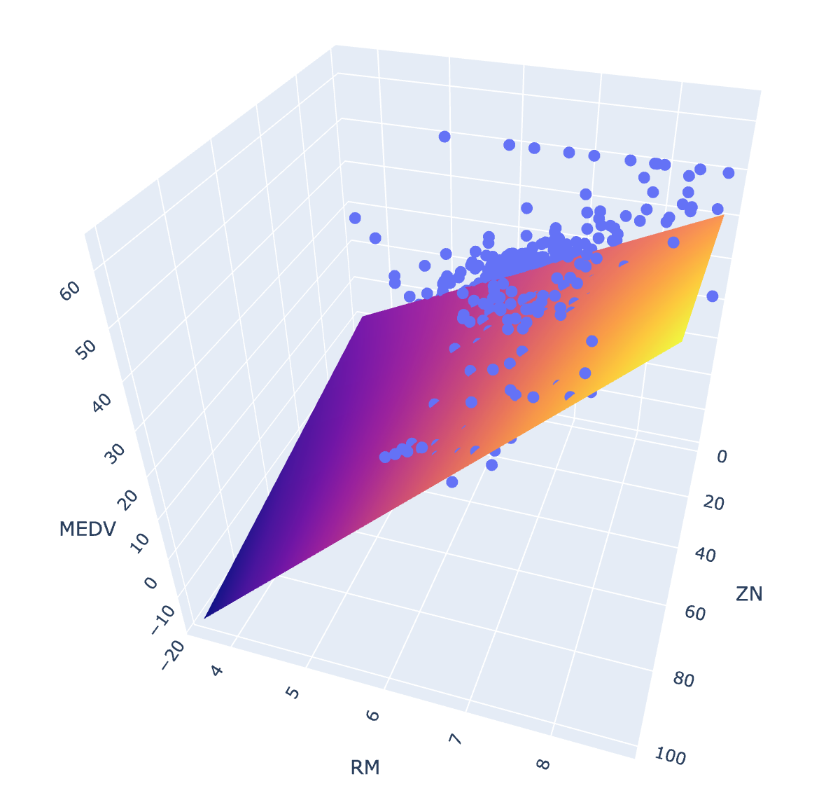
Just for fun - and because everyone loves a three-dimensional scatterplot - we can also view our regression models in 3D using plotly. Below, I create a 3D scatterplot for a simpler model with only a single interaction term and no polynomial terms.
import numpy as np
import plotly.express as px
import plotly.graph_objects as go

# Define mash size for prediction surface
mesh_size = .02

# Train model
model = smf.ols(formula="MEDV ~ ZN + RM + ZN:RM", data=boston_df)
result = model.fit()

# Define x and y ranges
# Note: y here refers to y-dimension, not response variable
x_min, x_max = boston_df["ZN"].min(), boston_df["ZN"].max()
y_min, y_max = boston_df["RM"].min(), boston_df["RM"].max()
xrange = np.arange(x_min, x_max, mesh_size)
yrange = np.arange(y_min, y_max, mesh_size)
xx, yy = np.meshgrid(xrange, yrange)

# Get predictions for all values of x and y ranges
pred = model.predict(params=result.params, exog=np.c_[np.ones(shape=xx.ravel().shape), xx.ravel(), yy.ravel(), xx.ravel()*yy.ravel()])

# Reshape predictions to match mesh shape
pred = pred.reshape(xx.shape)

# Plotting
fig = px.scatter_3d(boston_df, x='ZN', y='RM', z='MEDV')
fig.update_traces(marker=dict(size=5))
fig.add_traces(go.Surface(x=xrange, y=yrange, z=pred, name='predicted_MEDV'))
fig.show()
Potential pitfalls
Below, I’ll briefly discuss and explore some potential pitfalls of the linear regression model. I’ll attempt to quantify some of these potential issues, to see if they are truly problematic for my working example.
Non-linearity of the response-predictor relationships
I have already shown above a residual plot used to quantify non-linearity between the response and predictors. For comparison, below I’ll create the residual plot for the model above with the highest value of $R^2$. This model involves multiple polynomial terms and is non-linear by definition, but viewing its residual plot can still inform as to the overall model fit.
y = boston_df["MEDV"]
y_hat = result.predict()
resid = y - y_hat

sns.scatterplot(x=y_hat, y=resid).set(xlabel="Predicted Value",
                                      ylabel="Residual")
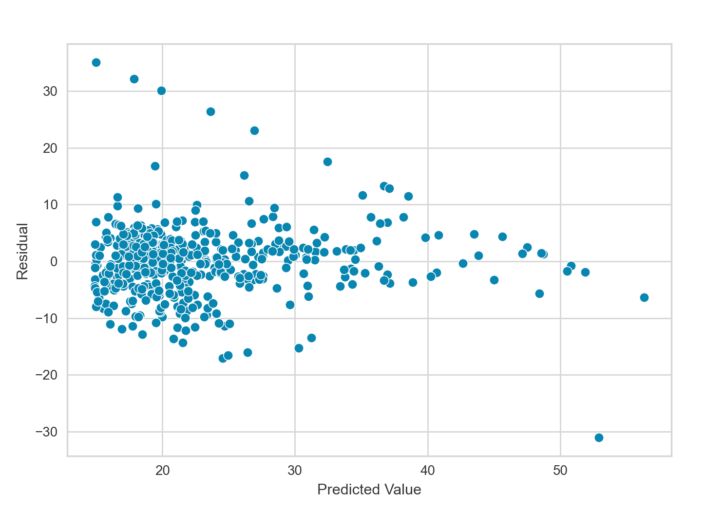
This most recent residual plot has less of a pattern than the one shown earlier, indicating the polynomial fit captures the overall relationship of the data better than the simpler model discussed earlier. If we ignore the diagonal line in the top right of the plot caused by the abundance of 0 ZN values, the residual plot looks quite ideal.
Correlation of error terms
When viewing the results of a linear regression fit, we should take care to also investigate if any correlation among the error terms is present.
Correlation of error terms - more often called serial correlation or autocorrelation in time series regression - can be particular problematic in that setting. In the time series regression setting, it can be useful to view a residual time series plot. Most of the residual values should be within a 95% confidence interval around 0. It is also useful to calculate the Durbin-Watson statistic, which is a test of significant residual autocorrelation at lag-1. When high autocorrelation is detected (e.g. a Durbin-Watson statistic below 1.6-1.8 or a lag-1 residual autocorrelation above 0.3-0.4), it can be useful to add new model terms, add seasonal adjustments to the model, or stationarize all predictor variables through differencing, logging or deflating.
In future posts, I’ll explore time-series regression in more depth.
In the current non-time series setting, we can diagnosis error term correlation by plotting the residuals versus predictor variables. In the ideal situation with no error term correlation, the residuals should be randomly and symmetrically distributed around zero.
import matplotlib.pyplot as plt

fig, axs = plt.subplots(nrows=2)
sns.scatterplot(x=boston_df["ZN"], y=resid, ax=axs[0]).set(ylabel="Residual")
sns.scatterplot(x=boston_df["RM"], y=resid, ax=axs[1]).set(ylabel="Residual")
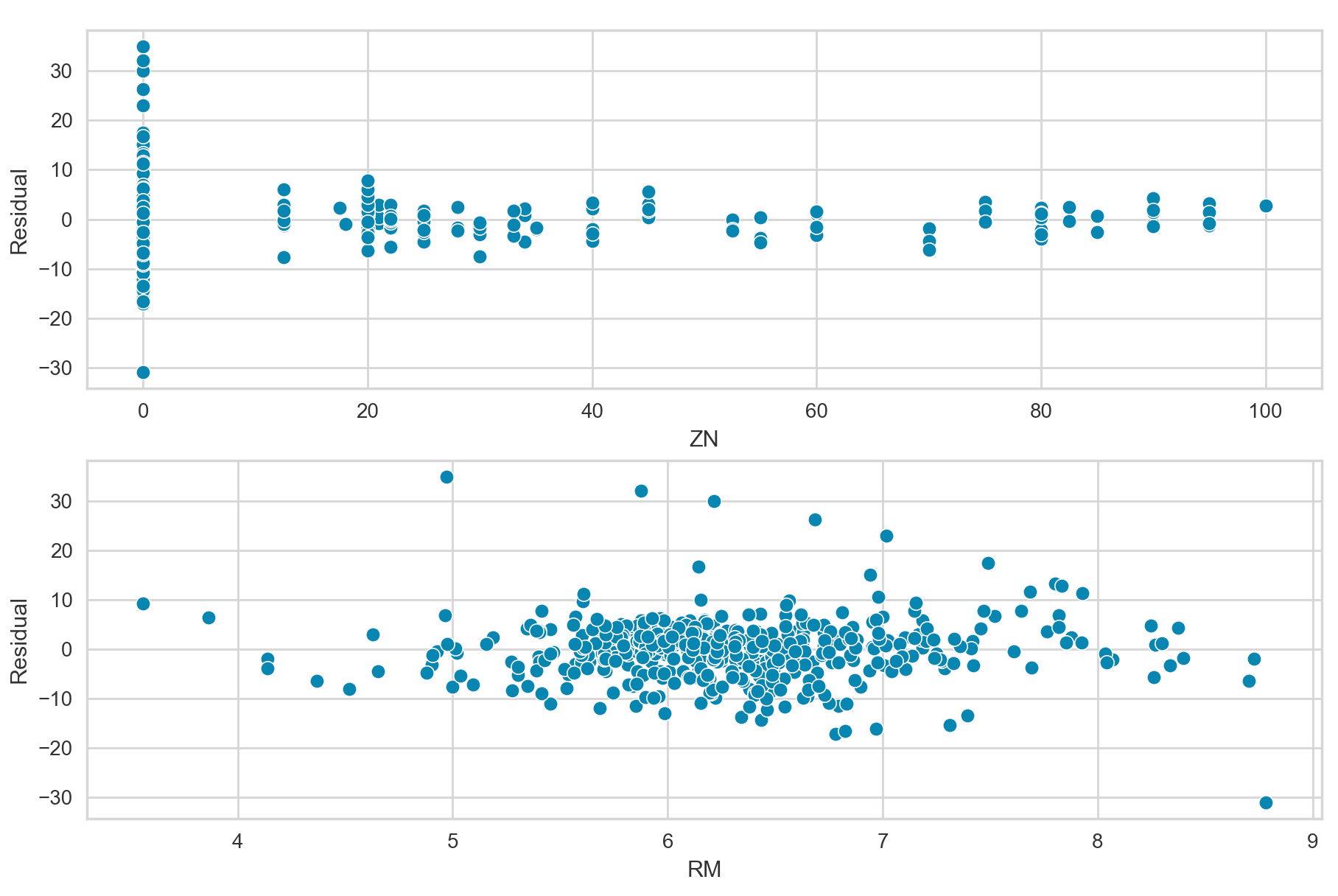
The above plots show the residuals versus the predictor variables ZN and RM, respectfully. Overall, these plots do not appear to show any strong patterns, and the residuals are mostly randomly and symmetrically distributed around zero.
Non-constant variance of error terms (heteroscedasticity)
Heteroscedasticity (sometimes spelled Heteroskedasticity) refers to the non-constant variance of the error terms of a model. It is often useful to visually inspect the residual plot for heteroscedasticity. From the above residual plot, we can see that the residual variance does seem to increased as the value of $\hat{y}$ increases, although the pattern isn’t obvious.
Instead of visually inspecting the residual plot for heteroscedasticity, it can be useful to quantify how constant the residual variance is via the Breusch-Pagan test. This test, developed in 1979, tests whether the variance of the errors from a linear regression is dependent on the values of the predictor variables. In this case, heteroscedasticity is present.
We can perform the Breusch-Pagan test via the statsmodels het_breuschpagan function.
>>> import statsmodels.stats.api as sms
>>> from statsmodels.compat import lzip

>>> returned_names = ['Lagrange multiplier statistic', 'p-value',
                      'f-value', 'f p-value']

>>> bp_test_results = sms.het_breuschpagan(resid, X_poly)
>>> lzip(returned_names, bp_test_results)
[('Lagrange multiplier statistic', 29.462789868830658),
 ('p-value', 1.8810315726665496e-05),
 ('f-value', 6.182684005037273),
 ('f p-value', 1.4192042140523905e-05)]
The p-value of the above test is approximately 1.88e-5, or 0.0000188. This p-value is significantly low, so we can reject the null hypothesis that the error terms are independent of the values of the predictor variables. Thus, we can conclude that heteroscedasticity is present, confirming our visual inspection.
Outliers
One method of quantifying outliers is by calculating the studentized residual of each point. The studentized residual is calculated by dividing each residual $e_i$ by its estimated standard error. We can use the outlier_test() method from statsmodel to calculate these values.
Below, I recreate the same model as above using the statsmodels formula interface, and then use the outlier_test() method to calculate the studentized residuals. After that, I remove the six data points with studentized residuals more extreme than -3 or 3, and then refit the model.
# Fitting model
model = smf.ols("MEDV ~ ZN + I(ZN**2) + RM + I(RM**2) + ZN*RM + I(ZN*RM**2)",
                data=boston_df)
result = model.fit()

# Getting studentized residuals
studentized_resids = result.outlier_test()

# Getting six data points with studentized residuals <-3 or >3
studentized_resids = \
    (studentized_resids
     .assign(student_resid_abs=abs(studentized_resids["student_resid"])))
outliers = \
    (studentized_resids
     .sort_values(by="student_resid_abs", ascending=False)
     .head(6))

# Removing these points from boston_df
boston_df_no_outliers = boston_df[~boston_df.index.isin(outliers.index)]


model_no_outliers = smf.ols("MEDV ~ ZN + ZN**2 + RM + I(RM**2) + ZN*RM + I(ZN*RM**2)",
                            data=boston_df_no_outliers)
result_no_outliers = model.fit()
result_no_outliers.summary()
After removing these 6 points, the $R^2$ statistic of the model jumps from .582 to 0.677, which is a notable improvement. Of course, in practice, care should be taken when removing outliers, and it should only be done within reason.
High leverage points
In contrast to outliers, high leverage points are those that have usual predictor values $x_i$. High level points can have drastic effects on model fit, so they are important to identify. We can calculate the leverage statistic to quantify the leverage of a point. However, it can be more useful to make use of statsmodels influence_plot method, which plots studentized residuals versus leverage.
Below, I’ll create such an influence plot.
model = smf.ols("MEDV ~ ZN + I(ZN**2) + RM + I(RM**2) + ZN*RM + I(ZN*RM**2)",
                data=boston_df)
result = model.fit()

sm.graphics.influence_plot(result, size=6)
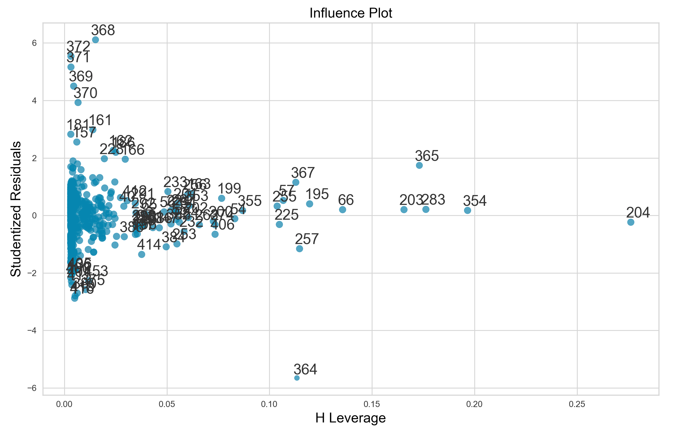
Points with a leverage statistic greater than the average are suspect. As such, data points 203, 283, 365, 354, and 204 clearly have high leverage and are likely strongly influencing our model fit.
Collinearity
In the regression context, collinearity among predictors can make it difficult to determine how each individual predictor is associated with the response, leading to reduced accuracy of the regression coefficient estimates
We can detect multicollinearity among our predictor variables by calculating each predictor’s variance inflation factor (VIF).
To do this, we can use the statsmodels variance_inflation_factor function.
>>> from statsmodels.stats.outliers_influence import variance_inflation_factor

>>> predictors = ["ZN", "ZN^2", "RM", "RM^2", "ZN*RM", "(ZN*RM)^2"]
>>> vifs = [variance_inflation_factor(exog=X_poly, exog_idx=i) for i in range(X_poly.shape[1])]

>>> pd.DataFrame(dict(predictor=predictors, vif=vifs))
   predictor          vif
0         ZN  2006.900702
1       ZN^2   123.275947
2         RM    96.513389
3       RM^2    11.965347
4      ZN*RM   139.454612
5  (ZN*RM)^2    98.352424
In general, a VIF above 5 or 10 indicates likely collinearity among our predictor variables. However, in this case, we have some pretty high VIF values. This occurrence is sometimes known as structural multicollinearity, and is a result of the polynomial terms in our regression model.
For a fairer comparison, we can view the VIF values when just ZN and RM are included.
>>> X = boston_df[["ZN", "RM"]].to_numpy()

>>> vifs = [variance_inflation_factor(exog=X, exog_idx=i) for i in range(X.shape[1])]
>>> predictors = ["ZN", "RM"]

>>> pd.DataFrame(dict(predictor=predictors, vif=vifs))
  predictor       vif
0        ZN  1.278583
1        RM  1.278583
From these last VIFs, we see that ZN and RM are not collinear, thus the accuracy of our coefficient estimates does not suffer.