Multiple linear regression #4

This post is the fourth in a series on the multiple linear regression model. In previous posts, I explored the topic, including methods of relaxing various assumptions made by the model. I also performed a comparison of Python’s scikit-learn and statsmodels libraries for multiple linear regression.

In this post, I’ll briefly discuss potential problems that can occur when fitting a multiple regression model to a particular dataset, including:

1. Non-linearity of the response-predictor relationships.
2. Correlation of error terms.
3. Non-constant variance of error terms.
4. Outliers.
5. High-leverage points.
6. Collinearity.

The structure of this post was influenced by the third chapter of An Introduction to Statistical Learning: with Applications in R by Gareth James, Daniela Witten, Trevor Hastie, and Robert Tibshirani.

Non-linearity of the response-predictor relationships

A key assumption made by the linear regression model is linearity between the predictors and response. If this assumption is not true for a particular dataset, then we should be skeptical of nearly all conclusions drawn from the model fit.

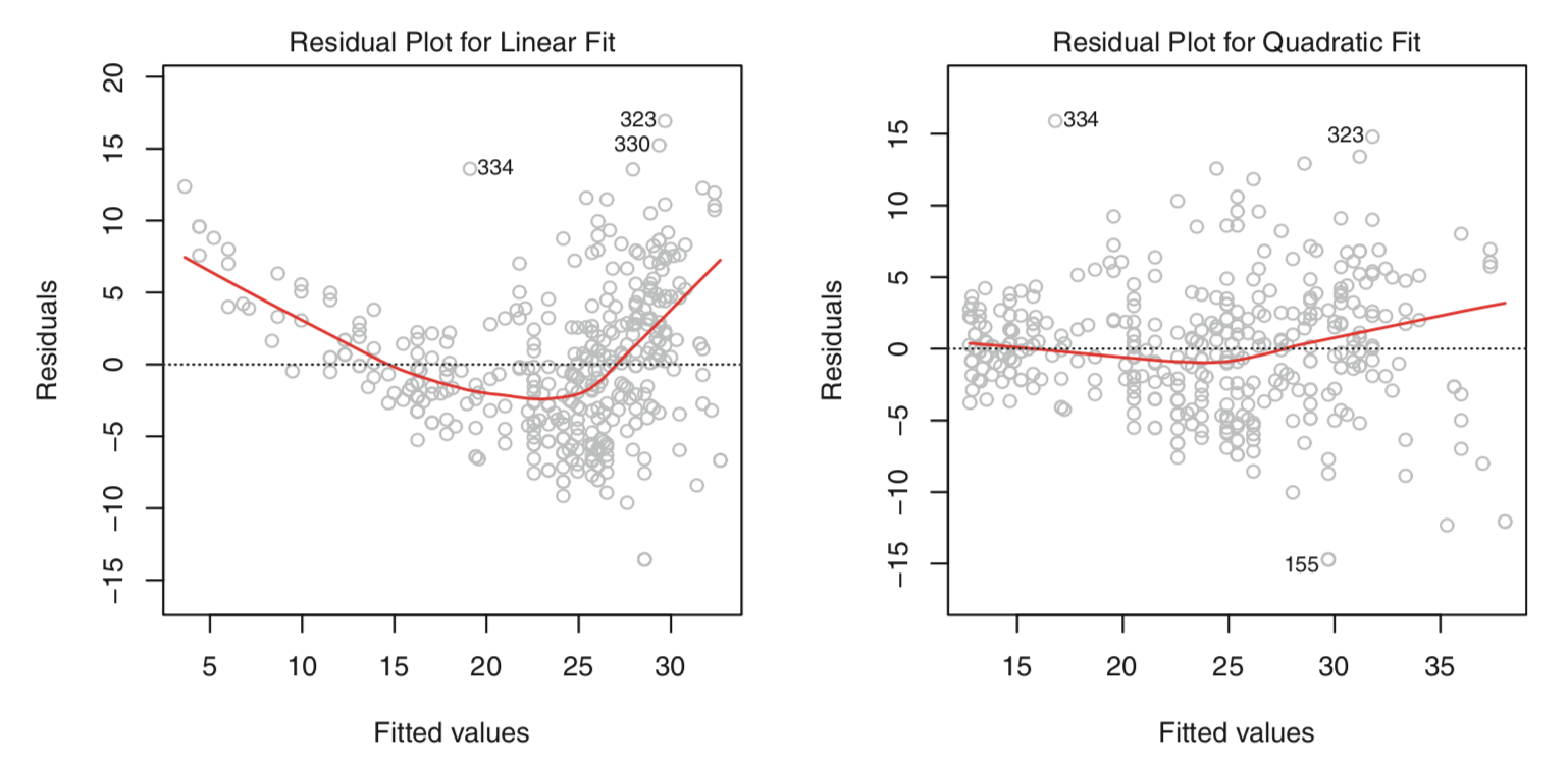
One method of identifying non-linearity is the residual plot. In the multiple regression context, we plot the residuals $e_i = y_i - \hat{y_i}$ versus the fitted values $\hat{y_i}$. If the true relationship is approximately linear, we should see little to no discernible pattern in the residual plot. If, however, a pattern in the residual plot is present, this is a strong indication that non-linearity does exist.

Source: Gareth James, Daniela Witten, Trevor Hastie, Robert Tibshirani. An Introduction to Statistical Learning: with Applications in R. New York: Springer, 2013.

Above are two residual plots. The left panel shows the resulting residual plot after a linear model fit, while the right panel shows the resulting residual plot after a quadratic model fit. In the left panel, there is a clear U-shape, indicating a strong non-linearity in the data. In contrast, in the right panel a much smaller pattern is present, indicating a quadratic term in the model improves the fit.

If the residual plot indicates a non-linear relationship in the data, a simple solution is to include a non-linear transformation of the predictors in the regression model. In future posts, I’ll explore more advanced non-linear approaches for addressing this issue.

Correlation of error terms

An assumption of the linear regression model is that the error terms, $\epsilon_1, \epsilon_2, \ldots, \epsilon_n$ are uncorrelated. In particular, the standard errors that are calculated for the regression coefficient estimates and fitted values are based on this assumption.

If the assumption of uncorrelated error terms is not true, then the estimated standard errors will tend to underestimate the true standard errors and the resulting confidence and prediction intervals will be narrower than they should be. Likewise, the associated p-values will also be lower than they should be, causing us to falsely conclude that a model term is significant. In general, correlated error terms can lead us to believe our model fit is better than it truly is.

Non-constant variance of error terms

Another important assumption of the linear regression model is that the error terms have a constant variance, $Var(\epsilon_i) = \sigma^2$. This constant error term variance is referred to as homoscedasticity. This assumption is key to standard errors, confidence intervals, and hypothesis tests associated with the model.

However, it is often the case that the variance of the error terms is non-constant, know as heteroscedasticity. In a residual plot, this can often be detected by the presence of a funnel shape. One possible solution to addressing this issue in practice is to transform the response variable using a concave function, such as $log \ Y$ or $\sqrt{Y}$. This transformation results in a greater amount of shrinkage of the larger response values, leading to a reduction in heteroscedasticity.

In the event where we can approximate the amount of variance of each response value, we can fit our model using weighted least squares. In the weighted least squares approach, each data point is multiplied by a nonnegative constant, or weight, that affects the influence that data point has on the model fit.

Outliers

An outlier is a point for which $y_i$ is far from the value predicted by the model. Outliers can occur for a variety of reasons. Depending on the outlier, it may or may not have a strong effect on the model fit. However, it can still have a strong effect on residual standard error (RSE) and the $R^2$ statistic. The RSE is also used in the computation of all confidence intervals and p-values associated with our model, so a single outlier can have drastic effects on the interpretability of our model fit.

Various methods can be used to detect the presence of outliers, including a simple residual plot. To quantify how extreme an outlier is, we can calculate its studentized residual by dividing each residual $e_i$ by its estimated standard error. In some contexts, a studentized residual is also known as a standardized residual.

High leverage points

In contrast to outliers, observations with high leverage have an unusual value of $x_i$. Observations with high leverage tend to have a substantial impact on the least squares regression line and may invalidate the entire fit. Thus, it’s important to identify high leverage observations.

In the simple linear regression context, high leverage points are fairly easy to determine. However, in the multiple linear regression context, detecting these points can be more challenging. This is because a high leverage observations may be within the range of each individual predictor’s values, but may be unusual within the full set of predictors.

To quantify an observation’s leverage, we calculate the leverage statistic. In the simple linear regression setting,

The leverage statistics $h_i$ is bounded between $1/n$ and $1$. Across all observations, it has mean $(p+1)/n$. Thus, if $h_i$ for a given observation is far greater than $(p+1)/n$, we might suspect that observations has high leverage.

Collinearity

Collinearity refers to the event in which two or more predictor variables are closely related to one another.

In the regression context, collinearity among predictors can make it difficult to determine how each individual predictor is associated with the response, leading to reduced accuracy of the regression coefficient estimates. This reduced accuracy can lead to enlarged standard errors $\hat{\beta_j}$, consequently leading to decreased $t$-statistics and increased p-values. Thus, in the presence of collinearity, we may fail to reject $H_0: \beta_j = 0$, indicating the power of the hypothesis test has been reduced.

One method of detecting collinearity among predictors is to look at the correlation matrix. However, this method is not robust to all possibly collinearities, as it is possible for collinearities to exist between three or more variables, even if no pair of variables has a particularly high correlation. This is referred to as multicollinearity.

Instead of inspecting the correlation matrix, a better approach is to calculate the variance inflation factor (VIF) for each predictor. The VIF is the ratio of the variance of $\hat{\beta_j}$ when fitting the full model divided by the variance of $\hat{\beta_j}$ if fit on its own. The smallest possible VIF is 1, and a value exceeding 5 or 10 indicates a problematic amount of collinearity. The VIF for each variable can be computed using the formula

where

is the $R^2$ from a regression of $X_j$ onto all the other predictors.

Once collinearity has been determined in the data, there are two simple solutions. The first is to drop one of the problematic variables. This can typically be done without much impact on the regression fit. The second solution is to combine the collinear variables into a single predictor, perhaps via averaging them after first standardizing.