This post is the second in a series on the multiple linear regression model. In a previous post, I introduced the model and much of it’s associated theory. In this post, I’ll continue exploring the multiple linear regression model with an example in Python, including a comparison of the scikit-learn and statsmodels libraries.
Introducing the example
As a working example, I’ll explore the effect weather had on airline flights leaving three New York City airports in 2013. In particular, I’ll join the airlines, flights, and weather datasets from the nycflights13 Python package and investigate the relationship wind speed, precipitation and visibility has on departure delay.
Preparing the data
Fortunately, the datasets I’ll be working with do not require much cleaning and organization before applying the model. After renaming the fields for clarity and converting the timestamp_hour fields to a datetime64 data type, I’ll join the dataframes via pandas’ merge and name it nyc. I’ll also drop missing values using pd.dropna(). In practice, a more thorough investigation into these missing values would be needed, but I’ll ignore this for demonstration purposes.
import pandas as pd
from nycflights13 import airlines, flights, weather


# Organizing airlines ---------------------------------------------------------

# Renaming fields for clarity
airlines = airlines.rename(columns={'carrier':'carrier_abbreviation',
                                    'name': 'carrier_name'})


# Organizing flights ----------------------------------------------------------

# Renaming fields for clarity
flights = flights.rename(columns={'dep_delay': 'departure_delay',
                                  'carrier': 'carrier_abbreviation',
                                  'origin': 'orig_airport',
                                  'time_hour': 'timestamp_hour'})

# Assigning timestamp_hour field to datetime type
flights = flights.assign(timestamp_hour=pd.to_datetime(flights.timestamp_hour, utc=True))


# Organizing weather ----------------------------------------------------------

# Renaming fields for clarity
weather = weather.rename(columns={'origin': 'orig_airport',
                                  'wind_speed': 'wind_speed_mph',
                                  'precip': 'precipitation_inches',
                                  'visib': 'visibility_miles',
                                  'time_hour': 'timestamp_hour'})

# Assigning timestamp_hour field to datetime type
weather = weather.assign(timestamp_hour=pd.to_datetime(weather.timestamp_hour, utc=True))


# Joining Data ----------------------------------------------------------------

# Joining
nyc = \
    flights \
    .merge(right=airlines, how='left', on='carrier_abbreviation') \
    .merge(right=weather, how='left', on=['orig_airport', 'timestamp_hour'])

# Selecting relevant fields and reordering
nyc = nyc[['timestamp_hour',
           'orig_airport',
           'carrier_name',
           'departure_delay',
           'wind_speed_mph',
           'precipitation_inches',
           'visibility_miles']]

# Dropping missing values
nyc = nyc.dropna()
At this point, the nyc dataframe has been created. A glimpse of the data structure can be seen below.
>>> nyc.info()
<class 'pandas.core.frame.DataFrame'>
Int64Index: 326915 entries, 0 to 336769
Data columns (total 7 columns):
 #   Column                Non-Null Count   Dtype
---  ------                --------------   -----
 0   timestamp_hour        326915 non-null  datetime64[ns, UTC]
 1   orig_airport          326915 non-null  object
 2   carrier_name          326915 non-null  object
 3   departure_delay       326915 non-null  float64
 4   wind_speed_mph        326915 non-null  float64
 5   precipitation_inches  326915 non-null  float64
 6   visibility_miles      326915 non-null  float64
dtypes: datetime64[ns, UTC](1), float64(4), object(2)
memory usage: 20.0+ MB

>>> nyc.head()
             timestamp_hour orig_airport            carrier_name  departure_delay  wind_speed_mph  precipitation_inches  visibility_miles
0 2013-01-01 10:00:00+00:00          EWR   United Air Lines Inc.              2.0        12.65858                   0.0              10.0
1 2013-01-01 10:00:00+00:00          LGA   United Air Lines Inc.              4.0        14.96014                   0.0              10.0
2 2013-01-01 10:00:00+00:00          JFK  American Airlines Inc.              2.0        14.96014                   0.0              10.0
3 2013-01-01 10:00:00+00:00          JFK         JetBlue Airways             -1.0        14.96014                   0.0              10.0
4 2013-01-01 11:00:00+00:00          LGA    Delta Air Lines Inc.             -6.0        16.11092                   0.0              10.0
Exploratory data analysis
Before diving into modeling, it’s good practice to perform some initial exploratory data analysis. I’ll use the seaborn data visualization library to create some plots.
Because the data is so large, I’ll take a small sample of 10,000 observations and create a pair plot.
import seaborn as sns

# Taking random sample, defining random_state for reproducibility
nyc_small = nyc.sample(n=10000, random_state=1234)

# Creating pair plot
sns.pairplot(nyc_small)\
    .fig.suptitle('10,000 Flights Leaving NYC, 2013: Pair Plot', y=1)
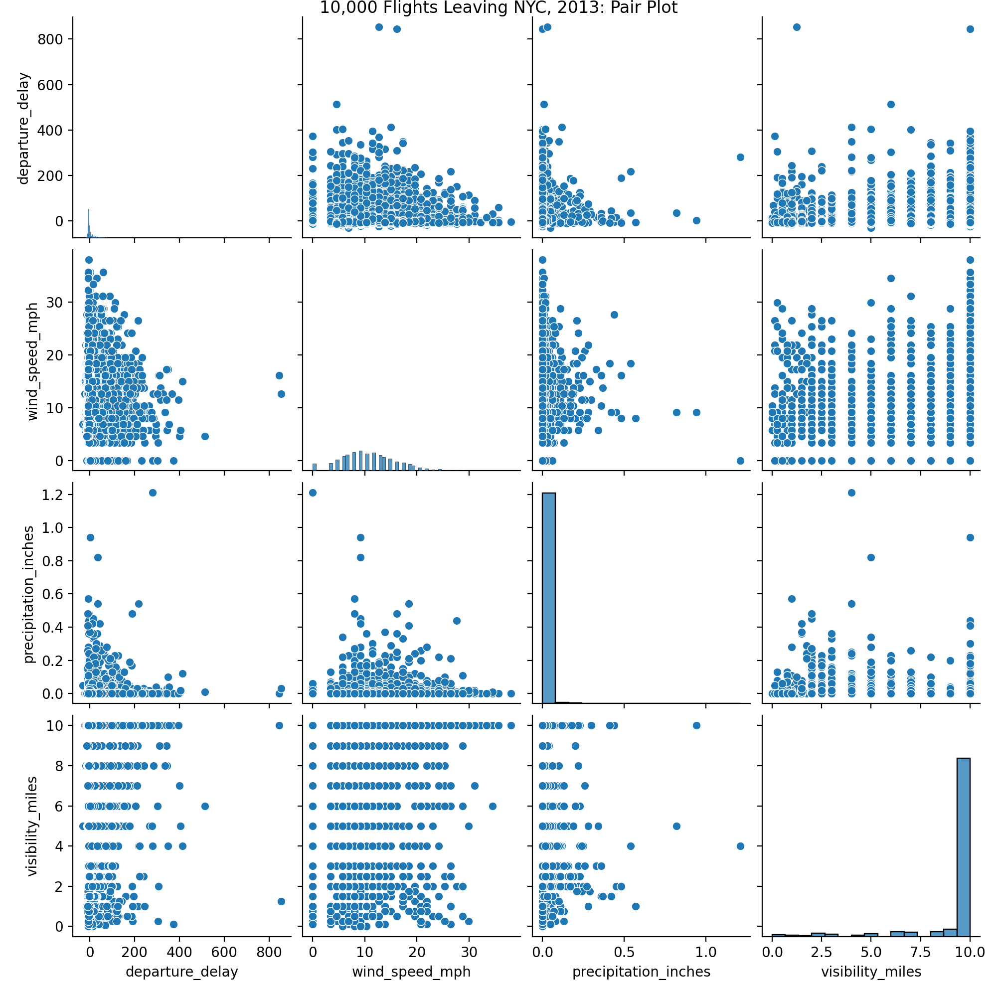
From the pair plot, it’s clear the data is quite noisy. However, we can still learn a thing or two from the plot. For example, most days in New York City tend to have good to mild weather with high visibility, low precipitation and moderate wind speeds. Also, from this small sample, no striking patterns or correlation stand out.
Perhaps instead of attempting to understand how these weather patterns affect individual departure delays, we should aggregate our data per hour and explore how average weather patterns affect average departure delays.
# Aggregating data per hour
nyc_per_hour = \
    nyc\
    .groupby("timestamp_hour")\
    .agg(mean_departure_delay=('departure_delay', 'mean'),
         mean_wind_speed_mph=('wind_speed_mph', 'mean'),
         mean_precipitation_inches=('precipitation_inches', 'mean'),
         mean_visibility_miles=('visibility_miles', 'mean'))\
    .reset_index()

sns.pairplot(nyc_per_hour)\
    .fig.suptitle('Flights Leaving NYC, 2013: Pair Plot of Average Per Hour Values', y=1)
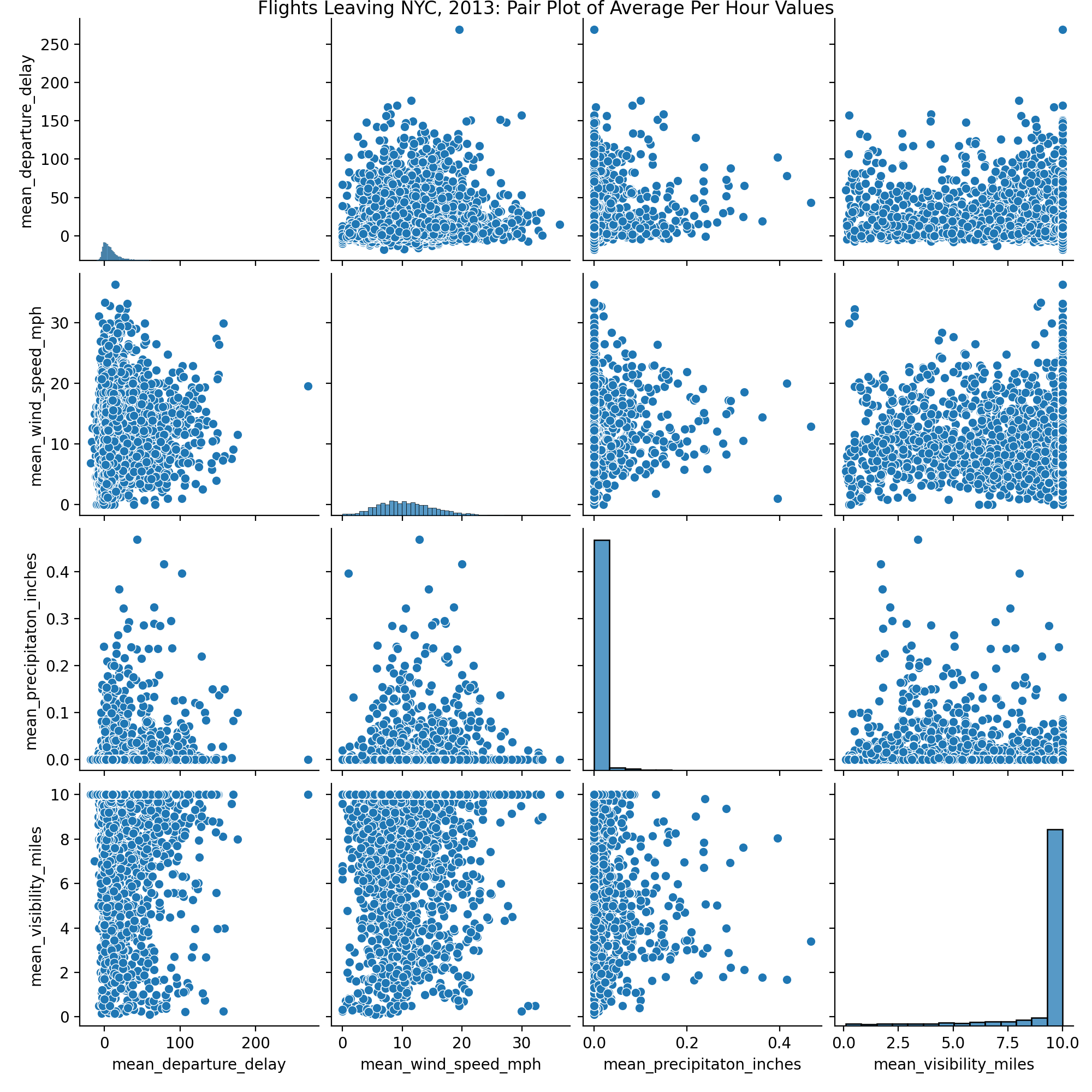
The pair plot for the new aggregated nyc_per_hour dataset is still quite busy. As a last plot, let’s create a correlation heatmap to confirm the lack of correlation among the variables.
import matplotlib.pyplot as plt
import numpy as np

labels =['Departure Delay', 'Wind Speed (MPH)', 'Precipitation (in)', 'Visibility (miles)']

sns\
    .heatmap(nyc_per_hour.corr(),
             mask=np.triu(np.ones_like(nyc_per_hour.corr())),
             annot=True,
             xticklabels=labels,
             yticklabels=labels)\
    .set_title('Correlation Heatmap of Average per Hour Values')

plt.xticks(rotation=45)
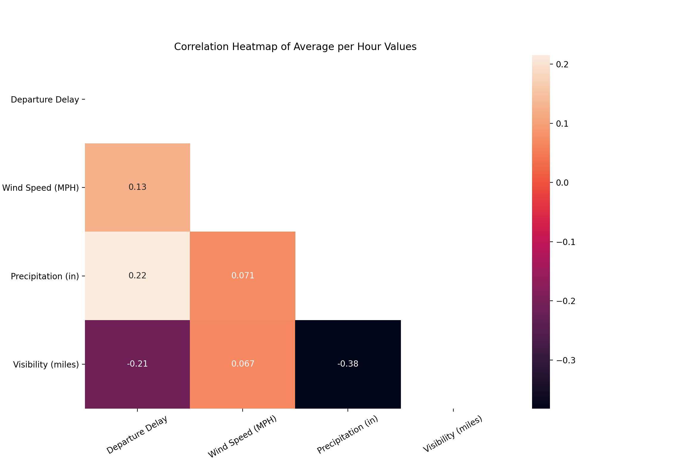
From the heatmap, we can see that the three predictor variables are mostly uncorrelated. For our multiple linear regression model, this is preferred. Multicollinearity among predictors can lead to spurious predictions and high variance among the regression coefficients. A variety of techniques can be helpful when dealing with mutlicollinearity among predictors, such as lasso regression and principal component analysis. These topics will be covered in more depth in later posts.
It is worth noting that there is a somewhat strong correlation between average precipitation and average visibility, with a Pearson correlation of -0.38. This isn’t surprising to see, as we might expect rainy days to have low visibility. For the purposes of this demonstration, I’ll ignore this multicollinearity.
From the heatmap as well, we can also see there is a small degree of correlation between average precipitation and average departure delay, with a Pearson correlation of 0.22, and a comparable negative correlation between average visibility and average departure delay with a Pearson correlation of -0.21.
Multiple linear regression via scikit-learn
After some exploratory analysis, we’re ready for modeling. I’ll first train the model using scikit-learn, and then train the same model using statsmodels. While scikit-learn is an excellent machine learning package, it isn’t intended for statistical inference. For this reason, I’ll explore the model summary of statsmodels in-depth to learn more about the regression in the next section.
Fitting the model via the scikit-learn API is quite simple. An estimator object is first created, and then is fit using the predictor variables X on the response variable y.
from sklearn.linear_model import LinearRegression

# Assign estimator
linear_reg = LinearRegression()

# Defining predictors and response
X = nyc_per_hour[['mean_wind_speed_mph', 'mean_precipitation_inches', 'mean_visibility_miles']]
y = nyc_per_hour['mean_departure_delay']

# Fitting model
linear_reg.fit(X=X, y=y)
After fitting the model, we can view the regression coefficients and intercept using the coef_ and intercept_ attributes. We could also perform prediction with the fitted model using the predict() method.
Of particular interest to this post is the score() method. For the linear regression model, this method returns $R^2$, or the coefficient of determination. This value indicates the proportion of variance explained by the model.
>>> linear_reg.score(X, y)
0.08295782066352853
For the particular fitted model above, the $R^2$ value is approximately 0.08, indicating about 8% of the total variance in the average flight departure delay is explained by the linear combination of average wind speed, average precipitation, and average visibility. Needless to say, that leaves a lot of variance unexplained, and our current linear model could almost certainly be improved upon.
In future posts, I’ll explore techniques that may better fit the data.
Multiple Linear Regression via statsmodels
Using the main statsmodels API provides a similar experience to scikit-learn’s API. To train a multiple linear regression model via statsmodels, we can use the OLS() function.
It is worth noting, statmodels does have a couple of nuances. First, by default, the OLS() function does not include an intercept. To include an intercept value in the model, we can use the add_constant() method.
Second, instead of the more common x and y parameter names, statsmodels uses exog and endog, referring to exogenous and endogenous.
Below, I’ll fit a multiple linear regression model using the main statsmodels API and the same X and y values defined above.
import statsmodels.api as sm

# Including constant term
X = sm.add_constant(X)

# Fitting model
linear_reg_sm = sm.OLS(endog=y, exog=X)
result = linear_reg_sm.fit()
In addition to the API interface above, statsmodels also provides a formula interface. This interface makes use of the patsy package under the hood, which, by the way, just might be the best package name I’ve ever heard of. As a former R user, this formula interface is quite familiar.
import statsmodels.formula.api as smf

# Fitting model
linear_reg_smf = smf.ols('mean_departure_delay ~ mean_wind_speed_mph + mean_precipitation_inches + mean_visibility_miles', data=nyc_per_hour)
result = linear_reg_smf.fit()

result.summary()
The summary() method can be used to view a useful summary table of the regression.
<class 'statsmodels.iolib.summary.Summary'>
"""
                             OLS Regression Results
================================================================================
Dep. Variable:     mean_departure_delay   R-squared:                       0.083
Model:                              OLS   Adj. R-squared:                  0.083
Method:                   Least Squares   F-statistic:                     207.5
Date:                  Tue, 12 Jan 2021   Prob (F-statistic):          7.29e-129
Time:                          20:30:14   Log-Likelihood:                -30586.
No. Observations:                  6886   AIC:                         6.118e+04
Df Residuals:                      6882   BIC:                         6.121e+04
Df Model:                             3
Covariance Type:              nonrobust
============================================================================================
                               coef    std err          t      P>|t|      [0.025      0.975]
--------------------------------------------------------------------------------------------
const                       24.4845      1.413     17.332      0.000      21.715      27.254
mean_wind_speed_mph          0.5334      0.049     10.949      0.000       0.438       0.629
mean_precipitation_inches  127.3312     11.298     11.270      0.000     105.183     149.479
mean_visibility_miles       -1.9262      0.143    -13.493      0.000      -2.206      -1.646
==============================================================================
Omnibus:                     4515.819   Durbin-Watson:                   0.385
Prob(Omnibus):                  0.000   Jarque-Bera (JB):            63194.997
Skew:                           2.986   Prob(JB):                         0.00
Kurtosis:                      16.586   Cond. No.                         683.
==============================================================================
Notes:
[1] Standard Errors assume that the covariance matrix of the errors is correctly specified.
"""
This summary table provides quite a bit of information. An interpretation of the $R^2$ value has already been discussed above. A few more statistics worth discussing here are the p-value of the F-statistic, indicated by Prob (F-statistic), and the p-values for the intercept and predictor terms, labeled as the P>|t| column.
The F-statistic can be used to determine if there exists any relationship between a predictor and the response. To simply look at the individual predictor p-values to determine if this relationship exists is flawed, as we would expect some individual variables to appear significant by chance alone, especially as the number of predictors in a model increases.
In this instance, the associated p-value of the F-statistic is approximately 7.29e-129, which is incredibly low. This p-value provides strong evidence that at least one predictor has an association with the response.
After determining that it is highly probable that a relationship does exist between at least one predictor and the response, we can investigate the individual predictor and intercept p-values. In the summary chart above, all four of these p-values are 0.000, indicating they are very close to zero. The pvalues method can be used to view the actual p-values.
>>> result.pvalues
const                       6.654574e-66
mean_wind_speed_mph         1.132716e-27
mean_precipitaton_inches    3.322614e-29
mean_visibility_miles       5.681725e-41
It is clear all of these p-values are quite small. Therefore, we can declare we have strong evidence that each of average wind speed, average precipitation, average visibility, and the intercept are significant and associated with average departure delay.
Lastly, I should discuss the implication of the very low $R^2$ and the very significant F-statistic and t-statistics.
With an ideal model fit, we would have simultaneously a high $R^2$ statistic, and significant F-statistics and t-statistics. However, in this instance, this is clearly not the case. Is this a problem? Should the results be thrown out? Not quite.
From the significant F-statistic and t-statistics, we have strong evidence that the predictor variables are associated with a change in average departure delay. We know this. From the low $R^2$ statistic, we also know that our multiple linear regression model does not capture the bulk of the average departure delay variance. So, our individual predictors are performing quite well, but our overall model is performing quite poorly. In general, this can be attributed to the wide variation in departure delay times in the data.
Other regression techniques - such as using interaction terms - might improve our fit on the data, and thus explain more of the variance in average departure delay. Similarly, including other predictor variables might also help in explaining more of the unexplained variance. In following posts, both of these topics will be explored.