Multiple linear regression is an extension of the simple linear regression model. In its simplest form it is a relatively inflexible method that can produce insightful results and accurate predictions under certain conditions. However, multiple linear regression has also been shown to be highly extensible, and many of these extensions (such as ridge regression, lasso regression, and logistic regression) vastly expand the usefulness and applicability of the linear regression paradigm.
In this post, I’ll briefly introduce the multiple linear regression model. I’ll discuss fitting of the model, estimating coefficients, assessing model accuracy, and considerations for prediction.
In future posts, I’ll compare and contrast the Python packages scikit-learn and statsmodels as they relate to statistical inference and prediction using the multiple linear regression model. I’ll also explore quantitative predictors, qualitative predictors and interaction terms.
The structure of this post was influenced by the third chapter of An Introduction to Statistical Learning: with Applications in R by Gareth James, Daniela Witten, Trevor Hastie, and Robert Tibshirani.
Multiple linear regression
In contrast to simple linear regression, multiple linear regression is able to handle multiple predictor variables, which is a much more common situation in practice. In general, the multiple linear regression model takes the form
\[\begin{aligned} Y = \beta_0 + \beta_1X_1 + \beta_2X_2 + ... + \beta_pX_p + \epsilon \end{aligned}\]where $X_j$ represents the $j$th predictor and $\beta_j$ quantifies the association between that variable and the response. $\beta_j$ is interpreted as the average effect on $Y$ of a one unit increase in $X_j$ holding all other predictors fixed.
Estimating coefficients
The multiple linear regression model is typically fit via the least squares method. This method approximates the values $\beta_0$, $\beta_1$,…, $\beta_p$ by determining the values $\hat{\beta_0}$, $\hat{\beta_1}$,…, $\hat{\beta_p}$ that minimize the sum of squared residuals
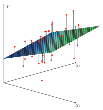
\[\begin{aligned} RSS = \sum_{i=1}^{n} (y_i - \hat{y_i})^2 \end{aligned}.\]For simple linear regression in a two-dimensional space, this fitting method results in a line passing through the data. However, for multiple linear regression, the method of least squares fitting results in a hyperplane that minimizes the squared distance between each point and the closest point on the plane. For the event where we have two predictor variables and one response variable, we can visualize the hyperplane as a two-dimensional plane in a three-dimensional space. In general, the multiple linear regression model is applicable to higher dimensional spaces as well.
 |
|---|
| Source: Gareth James, Daniela Witten, Trevor Hastie, Robert Tibshirani. An Introduction to Statistical Learning: with Applications in R. New York: Springer, 2013. |
Standard errors
After finding our estimated coefficients $\hat{\beta_0}$, $\hat{\beta_1}$,…, $\hat{\beta_p}$, it is natural to wonder how accurately each value estimates the true values $\beta_0$, $\beta_1$,…, $\beta_p$. In general, the standard error of the estimate can be calculated to answer this question. Continuing with the comparison to simple linear regression, the intercept estimate $\hat{\beta_0}$ and the coefficient estimate $\hat{\beta_1}$ under the simple linear regression model can be computed via the following formulas:
\[\begin{aligned} SE(\hat{\beta_0})^2 = \sigma^2\left[\frac{1}{n} + \frac{\bar{x}^2} {\sum_{i=1}^{n}(x_i-\bar{x})^2}\right], SE(\hat{\beta_1})^2 = \frac{\sigma^2}{\sum_{i=1}^{n}(x_i - \bar{x})^2} \end{aligned}\]where $\sigma^2 = Var(\epsilon)$.
Note, these standard error formulas assume that the errors $\epsilon_i$ for each observation are uncorrelated and have the same variance $\sigma^2$. This assumption is rare in practice, but these standard error estimations still turn out to be a good approximation. Similarly, in general, $\sigma^2$ is typically not known, but can be estimated from the data. This estimation is known as the residual standard error and is given by $RSE = \sqrt{RSS/(n-2)}$.
Confidence intervals and hypothesis testing
Returning to the multiple linear regression model, standard errors can also be used to computer confidence intervals and perform hypothesis tests. For linear regression, a 95% confidence interval for $\beta_j$ is approximately equivalent to
\[\begin{aligned} \hat{\beta_j} \pm 2 \cdot SE(\hat{\beta_j}) \end{aligned}.\]The most common hypothesis test involves testing the null hypothesis that there is no relationship between $X$ and $Y$. Mathematically, this is equivalent to testing
\[\begin{aligned} H_0: \beta_j = 0 \end{aligned}\]versus
\[\begin{aligned} H_a: \beta_j \neq 0 \end{aligned}.\]To test the null hypothesis, we need to quantify how far our estimated coefficient $\beta_j$ is from 0. This can be determined by calculating a t-statistic given by
\[\begin{aligned} t = \frac {\hat{\beta_j}-0} {SE(\hat{\beta_j})} \end{aligned}.\]This t-statistic is a measurement of the number of standard deviations that $\hat{\beta_j}$ is away from 0. From the Central Limit Theorem, we know that for large sample sizes, the t-distribution will approximate a Gaussian distribution, and thus we can calculate a p-value for $\hat{\beta_j}$. For p-values below a predefined significance level - commonly 0.05 or 0.01 - we reject the null hypothesis.
Assessing model accuracy
The quality of a multiple linear regression fit is typically assessed via two values: the residual standard error (RSE) and the $R^2$ statistic. These values are included as standard output in most statistical software, including Python’s statsmodels module and the base R distribution. In a future post, I’ll explore examples and discuss these values in detail, but for now I’ll constrain my discussion to only theory.
Residual standard error
The residual standard error was briefly introduced above in the context of calculating standard error values. RSE, as defined above, is a measure of the standard deviation of the irreducible error term $\epsilon$. If a model fit is quite accurate and predictions obtained from the model are very close to the true response values, RSE is quite small. However, is a model fit is poor and predictions obtained from the model are far from the true response values, we can expect RSE to be quite high. Thus, RSE is considered a measure of the lack of fit of the model.
Note, the RSE is measured in the units of $Y$, and what is considered high or low is dependent on the problem at hand.
$R^2$ statistic
The $R^2$ statistic, commonly called the coefficient of determination or coefficient of multiple correlation, is an alternative measure of model fit. In contrast to RSE which is measured in the units of $Y$, the $R^2$ statistic is a proportion. The $R^2$ statistic indicates the proportion of variance explained by the model and is independent of the scale of $Y$. $R^2$ is calculated via the formula
\[\begin{aligned} R^2 = \frac{TSS - RSS}{TSS} = 1 - \frac{RSS}{TSS} \end{aligned}\]where $TSS = \sum_(y_i - \bar{y})^2$ is the total sum of squares and is a measure of the total variance in the response $Y$.
The $R^2$ statistic measures the proportion of variability in $Y$ that can be explained using $X$. A value close to 1 indicates that a large proportion of the variability in the response has been explained by the regression, while a value close to 0 indicates that the regression did not explain much of the variability in the response. A low $R^2$ value can occur when a linear model is not a good approximation of the data, or the variance of $\epsilon$ is inherently high, or both.
An extension of the $R^2$ statistic known as adjusted $R^2$ and denoted $R_{adj}^2$ will be discussed in a future post.
Determining if a relationship exists between $X$ and $Y$
A question we have yet to explore is that of whether there exists a relationship between the response and predictor variables. It might be tempting to use the individual predictor p-values discussed above to make this assessment and claim that if any individual predictor p-values are small, then at least one of the predictors is related to the response. However, this logic is flawed, especially when the number of predictors $p$ is large. As the number of predictors increases, the chance that the p-value of a single predictor will appear significant increases, even if there is no true association between the predictors and the response.
Fortunately, the F-statistic does not suffer from this problem, as it adjusts for the number of predictors.
Mathematically, determining if a relationship exists between the response and predictor variables is equivalent to the null hypothesis
\[\begin{aligned} H_0: \beta_1 = \beta_2 = ... = \beta_p = 0 \end{aligned}\]versus the alternative
\[\begin{aligned} H_a: \text{at least one } \beta_j \text{ is non-zero}. \end{aligned}\]This hypothesis test is performed by calculating the F-statistic,
\[\begin{aligned} F = \frac{(TSS - RSS)/p}{RSS/(n-p-1)} \end{aligned}\]If the assumptions of the linear model are correct, we can show that
\[\begin{aligned} E\{RSS/(n-p-1)\} = \sigma^2 \end{aligned}\]and that, provided $H_0$ is true,
\[\begin{aligned} E\{(TSS - RSS)/p\} = \sigma^2, \end{aligned}\]where $E\{X\}$ indicates the expected value.
When there is no relationship between the response and the predictors, we expect the F-statistic to be close to 1. However, when $H_a$ is true, then $E\{(TSS - RSS)/p\} > \sigma^2$, and we expect F to be greater than 1.
To determine whether to reject the null hypothesis, we can calculate a p-value from the resulting F-statistic. When $H_0$ is true and either the errors $\epsilon_i$ have a normal distribution, or the sample size $n$ is large, the F-statistic follows an F-distribution. Depending on the calculated p-value, we can either reject the null hypothesis and claim there is a relationship between the response and the predictors, or not reject the null hypothesis and make no such claim.
In the event where the F-statistic is low and we cannot claim that a relationship exists between the response and the predictors, we should not interpret any individual predictor p-values as significant.
Variable selection
If, after fitting a multiple linear regression model and calculating the F-statistic and associated p-values, we determine that at least one of the predictors is related to the response, the natural progression is to determine which predictor variables are actually associated with the response. It can be informative to look at the individual p-values, but as discussed above, this can be problematic when $p$ is large.
Determining which predictors are associated with the response, such that a single model can be fit with only these predictors is referred to as variable selection. In future posts, I will discuss this topic in more depth, so for now I will only briefly introduce a variety of methods.
When $p$ is small or domain knowledge about the problem is available, it may be feasible to fit multiple models, each containing a different subset of the predictors. When this is possible, a variety of statistics can be used to determine the quality of a model. Example of these statistics include Mallow’s Cp, Akaike information criterion (AIC), Bayesian information criterion (BIC) and adjusted $R^2$.
As $p$ increases, the model space grows exponentially and thus trying out many predictor combinations is infeasible. When this is the case, a variety of methods exist to automate and efficiently choose a smaller set of models to consider. A few of these methods are forward selection, backward selection and mixed selection.
Many other techniques exist as well to perform variable and model selection. Examples of such techniques are ridge regression, lasso regression, and principal component analysis
Considerations for prediction
Once a multiple linear regression model has been fit, it is trivial to predict the response $Y$. However, there are three types of uncertainty associated with this prediction we should be aware of.
Reducible error
The least squares plane
\[\begin{aligned} \hat{Y} = \hat{\beta_0} + \hat{\beta_1}X_1 + \hat{\beta_2}X_2 + ... + \hat{\beta_p}X_p \end{aligned}\]is only an estimate for true population regression plane
\[\begin{aligned} f(X) = \beta_0 + \beta_1X_1 + \beta_2X_2 + ... + \beta_pX_p \end{aligned}\]The coefficient estimates $\hat{\beta_0}$, $\hat{\beta_1}$,…, $\hat{\beta_p}$ will have some inaccuracies and is thus related to the reducible error. That is, it might be possible to estimate the true population regression plane more accurately under different conditions. For example, if we had more data, this might lead to a more accurate estimation. To quantify this error, we can calculate a confidence interval that determines how close $\hat{Y}$ will be to $f(X)$.
Model bias
Another source of potentially reducible error is model bias. In practice, assuming a linear model for $f(X)$ is almost always an approximation. Thus, the assumed linear model may be biased and perhaps a better model could reduce the error.
Irreducible error
Lastly, the third type of prediction uncertainty is related to the random error $\epsilon$. In the extreme event where we knew $f(X)$ exactly, we would still not be able to perfectly predict the response value. We refer to this as the irreducible error. To quantify how much $Y$ will vary from $\hat{Y}$, we use prediction intervals. Because prediction intervals incorporates both the reducible error and the irreducible error, they will always be larger than confidence intervals.