In a previous post I introduced the concept of cross-validation as a resampling technique. In particular, cross-validation is useful for estimating the test error of a particular model fit in order to evaluate its performance, or to decide on an optimal level of flexibility. In addition, cross-validation can also be used to select an ideal model among many potential models by comparing the estimated test errors among these models.
Depending on the problem and data at hand, it is sometimes ideal to first spit the available data into training and test sets, and then perform cross-validation on only the training set, and then use the test set for reporting, as this test set will contain data that has not influenced model training at all. Typically, the mean and standard deviation of the test error is reported.
In the below examples, I am only interested in the various cross-validation procedures, and will thus not first split my data into training and test sets. Instead, I will treat my entire dataset as a training set, and will draw various training and validation sets, where the validation set is drawn from the training set.
In a future post, I will explore nested cross-validation, which is a technique used to simultaneously perform model hyperparameter turning and evaluation.
Iris dataset
For the below examples, I will train a number of classifiers on the well known Iris dataset. The Iris dataset presents a simple and easy classification task, and is ubiquitous across machine-learning examples.
Let’s first create a simple scatter plot of the Iris data to visualize the three target classes.
import pandas as pd
import seaborn as sns
from sklearn.datasets import load_iris

# Loading Iris as pandas DataFrame
iris = load_iris(as_frame=True)

# Creating DataFrame to match up target label with target_name
iris_target_names = pd.DataFrame(data=dict(target=[0, 1, 2],
                                           target_name=iris.target_names))

# Merging predictor and response DataFrames, via left join
data = (iris["frame"]
        .merge(right=iris_target_names,
               on="target",
               how="left"))

# Creating scatter plot
sns.scatterplot(x="sepal length (cm)",
                y="sepal width (cm)",
                hue="target_name",
                data=data)
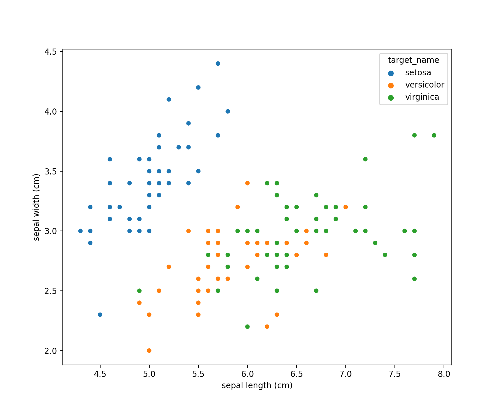
Note the Iris dataset contains four predictor fields in total. petal length(cm) and petal width(cm) are not shown on the above two-dimensional scatter plot.
Validation set approach
First, let’s explore the simple validation set approach. For detail on this approach, please see my earlier post.
Using scikit-learn, we can split our data into training and test sets using train_test_split function. Note, under this simple approach, the terms validation set and test set of often used interchangeable. We’ll train our classifier using the method of linear discriminant analysis.
from sklearn.discriminant_analysis import LinearDiscriminantAnalysis
from sklearn.model_selection import train_test_split

# Loading Iris again, returning X and y as NumPy arrays
X, y = load_iris(return_X_y=True)

# Simple validation set split
X_train, X_test, y_train, y_test = train_test_split(X, y,
                                                    test_size=0.25,
                                                    random_state=1234,
                                                    shuffle=True)

# Initializing LDA estimator and fitting on training observations
lda = LinearDiscriminantAnalysis()
lda.fit(X=X_train, y=y_train)
Note, under the hood, train_test_split is simply a wrapper around the scikit-learn ShuffleSplit and StratifiedShuffleSplit classes.
Now that we’ve trained our model, we use the predict and score methods to see the class predictions and calculate the correct classification rate, or accuracy, respectively.
lda.predict(X_train)  # predictions on training set
lda.predict(X_test)   # predictions on test set

lda.score(X=X_train, y=y_train)  # accuracy on training set
lda.score(X=X_test, y=y_test)    # accuracy on test set
On the training set, our accuracy is approximately 98.214%, while on the test set it is approximately 97.368%. Since the Iris classification task is so easy, these high accuracy rates (and corresponding low error rates) aren’t surprising. On more challenging classification tasks in practice, we would expect much higher error rates.
Note as well, under a different random validation set split, we would expect different training and error rates.
$k$-fold and stratified $k$-fold cross-validation
Next, let’s explore $k$-fold cross-validation. $k$-fold cross-validation and it’s related techniques are probably the most popular techniques used in practice for model assessment and selection. For a detailed introduction to the $k$-fold cross-validation, please refer to my earlier post on the concept.
A related technique to $k$-fold cross-validation is stratified $k$-fold cross-validation. Stratified $k$-fold cross validation is similar to $k$-fold cross-validation, except the observations in each of the $k$ folds are selected such that class labels of a qualitative response are roughly equally distributed. This is particularly useful for classification tasks where the class labels are highly imbalanced.
scikit-learn’s cross_val_score
We can use scikit-learn’s cross_val_score function to perform these types of cross-validation techniques. cross_val_score will perform $k$-Fold cross validation, unless the estimator is a classifier and y is binary or multiclass, in which case stratified $k$-fold cross-validation is used.
Using our same lda estimator from above, we can use cross_val_score to perform stratified 10-fold cross-validation.
>>> from sklearn.model_selection import cross_val_score

>>> scores = cross_val_score(estimator=lda, X=X, y=y, cv=10)
>>> scores

array([1.        , 1.        , 1.        , 1.        , 0.93333333,
       1.        , 0.86666667, 1.        , 1.        , 1.        ])
Note, the ten returned values are the accuracy rates for the model trained on the other nine folds, and evaluated on the particular validation fold. By default, cross_val_score performs 5-fold cross-validation using cv=5.
We can also easily calculate the mean and standard deviation of these ten cross-validation scores.
scores.mean()  # 0.98
scores.std()   # 0.0356
Under the hood, cross_val_score calls scikit-learn’s KFold or StratifiedKFold classes to perform the cross-validation. We could have performed the same cross-validation procedure as above using the below code.
from sklearn.model_selection import StratifiedKFold

cv_stratified_k_fold = StratifiedKFold(n_splits=10, shuffle=False)
cross_val_score(estimator=lda, X=X, y=y, cv=cv_stratified_k_fold)
In the regression setting, we can use the KFold class in an analogous manner.
scikit-learn’s cross_validate
In addition to cross_val_score, scikit-learn also offers the cross_validate function. This function supports evaluating multiple specified scoring metrics, and it returns a dictionary containing fit times, score times, test scores, and optionally training scores. The time measures are returned in units of seconds.
from sklearn.model_selection import cross_validate

scores = cross_validate(estimator=lda,
                        X=X,
                        y=y,
                        cv=10,
                        scoring=("roc_auc_ovo", "accuracy"),
                        return_train_score=True)
A list of supported scoring metrics can be found here.
The Python standard library pprint is useful for viewing dictionary objects like scores.
>>> from pprint import pprint

>>>pprint(scores)

{'fit_time': array([0.00120902, 0.04706788, 0.00307202, 0.00163078, 0.00100708,
       0.00134993, 0.00214291, 0.00090027, 0.00096679, 0.00087285]),
 'score_time': array([0.00728393, 0.07550716, 0.005898  , 0.00772309, 0.00524998,
       0.00416422, 0.00359702, 0.00362277, 0.00341129, 0.00327492]),
 'test_accuracy': array([1.        , 1.        , 1.        , 1.        , 0.93333333,
       1.        , 0.86666667, 1.        , 1.        , 1.        ]),
 'test_roc_auc_ovo': array([1.        , 1.        , 1.        , 1.        , 1.        ,
       1.        , 0.98666667, 1.        , 1.        , 1.        ]),
 'train_accuracy': array([0.97777778, 0.97777778, 0.97777778, 0.97777778, 0.98518519,
       0.97777778, 0.99259259, 0.97777778, 0.97777778, 0.97777778]),
 'train_roc_auc_ovo': array([0.99884774, 0.99884774, 0.99884774, 0.99901235, 0.99917695,
       0.99934156, 0.99983539, 0.99917695, 0.99901235, 0.99901235])}
Comments on repeated $k$-fold cross-validation
At this point, it would be useful to briefly discuss the repeated $k$-fold cross-validation technique, and the lack of use it provides.
Repeated $k$-fold cross-validation refers to a technique in with the $k$-fold cross-validation method is repeated multiple times. Since $k$-fold cross-validation creates random folds of the data and returns an estimation of the test error, repeated $k$-fold cross-validation returns multiple estimates of the test error, each created with different random folds. After all the repeated cross-validation test error rates are returned, summary statistics such as the mean and standard deviation of all test error estimates are often reported.
This technique and the stratified variant of it are supported in scikit-learn via the RepeatedKFold and RepeatedStratifiedKFold classes.
While repeated $k$-fold cross validation may seem like an attractive method to produce a more accurate test error estimate, it has been found to be not useful in practice and often misleading.
In a 2012 paper by Belgian researchers Gitte Vanwinckelen and Hendrik Blockeel, it was argued that when performing cross-validation for model assessment and selection, we are interested in the predictive accuracy of our model on a sample $S$ taken from a population $P$. The authors denote this value as $\sigma_2$ and contrast it with $\sigma_1$, the mean predictive accuracy of our model taken over all data sets $S’$ of the same size as $S$ taken from $P$.
$\sigma_2$ has both bias (because $S$ is a subset taken from $P$; a new subset $S_1$ would be different) and has high variance (because of the randomly selected $k$ folds used to estimate the test error rate).
The authors argue that repeating the $k$-fold cross-validation process can reduce the variance, but not the bias. Instead, the repeated $k$-fold cross-validation process produces an accurate estimate of the mean of all $k$-fold cross-validation test error estimates, across all possible $k$-fold cross-validations, denoted $\mu_k$. However, we are interested in $\sigma_2$, and $\mu_k$ is not necessarily an accurate estimate of $\sigma_2$.
Not useful example of repeated $k$-fold cross-validation
After reading the above paper, I was still interested in applying the method of repeated $k$-fold cross-validation for my own knowledge and exploration. With the understanding that the below method does not produce meaningful results in practice, below is an example demonstrating how to apply repeated stratified $k$-fold cross-validation to compare four classifiers.
First, let’s initialize the RepeatedStratifiedKFold object. We’ll perform 10-fold cross-validation across 5 repeats.
from sklearn.model_selection import RepeatedStratifiedKFold

cv_repeated_stratified_k_fold = RepeatedStratifiedKFold(n_splits=10,
                                                        n_repeats=5,
                                                        random_state=1234)
Next, let’s perform this cross-validation technique to compare the classification results of linear discriminant analysis, quadratic discriminant analysis, logistic regression, and quadratic logistic regression.
I’ll create a separate scikit-learn Pipeline for each model first.
For the particular models chosen below, scaling our features will not affect the results. However, for demonstration purposes, I decided to scale the features in each pipeline. I also found the LDFGS solver did not converge for the quadratic logistic regression model without first scaling the features.
Note, the logistic regression and quadratic logistic regression models below will be one-vs-rest multi-class classifiers, since our target in the Iris dataset has three distinct levels.
from sklearn.discriminant_analysis import QuadraticDiscriminantAnalysis
from sklearn.linear_model import LogisticRegression
from sklearn.pipeline import Pipeline
from sklearn.preprocessing import PolynomialFeatures, StandardScaler

# Creating individual pipelines for each model
pipeline_lda = \
    ("LDA", (Pipeline([
        ("standard_scaler", StandardScaler()),
        ("lda", LinearDiscriminantAnalysis())
    ])))

pipeline_qda = \
    ("QDA", Pipeline([
        ("standard_scaler", StandardScaler()),
        ("qda", QuadraticDiscriminantAnalysis())
    ]))

pipeline_log_reg = \
    ("Logistic Regression", Pipeline([
        ("standard_scaler", StandardScaler()),
        ("log_reg", LogisticRegression(penalty="none"))
    ]))

pipeline_quadratic_log_reg = \
    ("Quadratic Logistic Regression", Pipeline([
        ("standard_scaler", StandardScaler()),
        ("polynomial_features", PolynomialFeatures(degree=2, interaction_only=False)),
        ("logistic_regression", LogisticRegression(penalty="none"))
    ]))
Next, we’ll create a list of our Pipelines, and loop through them to calculate the repeated stratified $k$-fold cross-validation test error rates. Within the loop, the results will be organized into a single pandas DataFrame.
# Initializing DataFrame for results
results = pd.DataFrame()

# Looping through pipelines, storing results
for pipe, model in pipelines:

    # Getting cross validation scores
    cv_scores = cross_val_score(model, X, y, cv=cv_repeated_stratified_k_fold)

    # Calculating mean CV scores (approximation for mu_1 in paper's notation)
    cv_scores_mean = pd.DataFrame(data=cv_scores.reshape(10, 5)).mean()

    # Organizing results into DataFrame
    results_per_model = pd.DataFrame(data=dict(mean_cv_score=cv_scores_mean,
                                               model=pipe,
                                               repeat=["Repeat " + str(i) for i in range(1, 6)]))

    # Concatenating results
    results = pd.concat([results, results_per_model])
Our results object contains five averaged cross-validation scores (one for each repeat) for each of the four models.
>>> results
   mean_cv_score                          model    repeat
0       0.973333                            LDA  Repeat 1
1       0.966667                            LDA  Repeat 2
2       0.973333                            LDA  Repeat 3
3       0.986667                            LDA  Repeat 4
4       1.000000                            LDA  Repeat 5
0       0.960000                            QDA  Repeat 1
1       0.966667                            QDA  Repeat 2
2       0.953333                            QDA  Repeat 3
3       0.986667                            QDA  Repeat 4
4       1.000000                            QDA  Repeat 5
0       0.953333            Logistic Regression  Repeat 1
1       0.953333            Logistic Regression  Repeat 2
2       0.980000            Logistic Regression  Repeat 3
3       0.980000            Logistic Regression  Repeat 4
4       1.000000            Logistic Regression  Repeat 5
0       0.946667  Quadratic Logistic Regression  Repeat 1
1       0.906667  Quadratic Logistic Regression  Repeat 2
2       0.926667  Quadratic Logistic Regression  Repeat 3
3       0.940000  Quadratic Logistic Regression  Repeat 4
4       0.960000  Quadratic Logistic Regression  Repeat 5
Lastly, we can plot our results via a boxplot.
(sns
 .boxplot(data=results, x="model", y="mean_cv_score")
 .set(title='Model Comparison via \n Repeated Stratified k-Fold Cross Validation',
      xlabel="Model",
      ylabel="Mean Cross-Validation Score"))
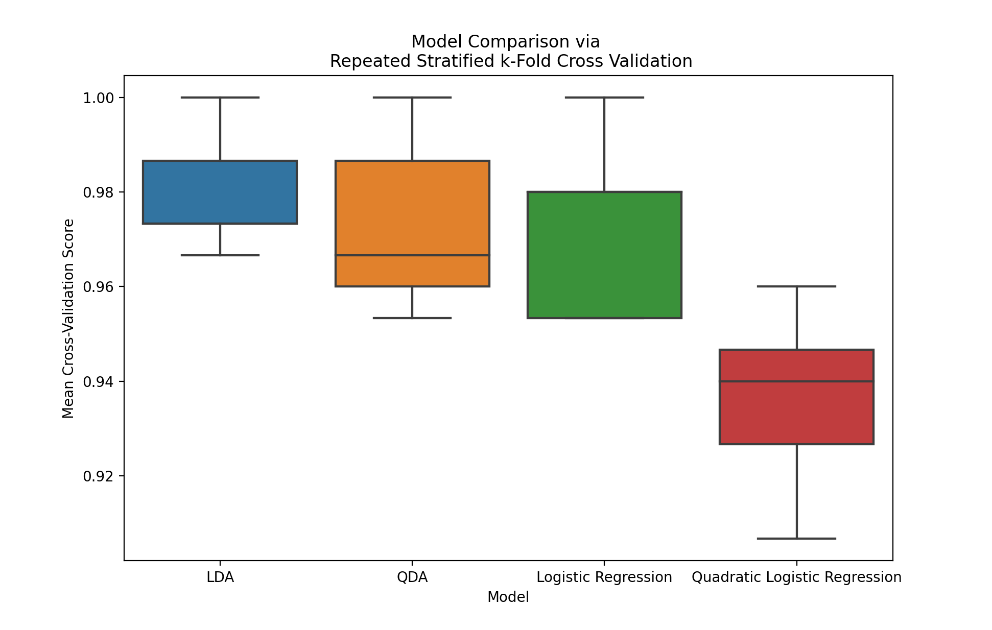
Due to the easy nature of this classification task, all of our accuracy values are quite high. It does appear that the quadratic logistic regression model is (not surprisingly) overfitting the data, and is performing worse on the validation sets.
Leave-one-out cross validation
To implement leave-one-out cross-validation (LOOCV), we can use scikit-learn’s LeaveOneOut class. For a more detailed introduction to LOOCV, please refer to my previous post on cross-validation.
from sklearn.model_selection import LeaveOneOut

cv_loo = LeaveOneOut()
scores = cross_val_score(lda, X, y, cv=cv_loo)
scores.mean()  # 0.98
Other cross-validation techniques
Lastly, I wanted to briefly discuss some other cross-validation techniques supported by scikit-learn.
GroupKFold
The GroupKFold class is similar to the regular KFold class, except all observations for a unique group is guaranteed to never be in both the training and validation sets. That is, all observations for a particular group will appear in either the training or validation set per cross-validation iteration, but not both.
This technique is useful when the information about a particular group should remain together for model training, and then the model should be assessed on unseen groups.
For example, if we have data on various customers (with multiple observations per customer) and we are hoping to predict whether a customer will churn or not, it might be useful to use all observations about various customers to train the model, and to then predict churn on unseen observations related to other customers.
TimeSeriesSplit
The TimeSeriesSplit class can be used to perform cross-validation on time series observations observed at fixed time intervals.
Time series data is characterized by correlation of observations that are near in time (known as autocorrelation). However, standard cross-validation techniques such as $k$-fold cross-validation assume the observations are independent and identically distributed. Thus, using these standard techniques on time series data would create unrealistic correlation between training and validation observations, and would result in poor generalized test error estimates.
Therefore, with time series data, we must evaluate our models using “future” observations that were not used to train the model.
The TimeSeriesSplit class achieves this by returning the first $k$ folds as a training set and the $k+1$th fold as a validation set. Then, for each cross-validation iteration, successive training sets are supersets of earlier training sets, and the new validation set becomes the next fold in temporal order.
Other techniques
In addition to the techniques discussed above, a variety of other scikit-learn cross-validation methods can be found here.